Response_Point_09-2
Last updated: 2020-09-23
Checks: 6 1
Knit directory: Comparative_eQTL/analysis/
This reproducible R Markdown analysis was created with workflowr (version 1.5.0). The Checks tab describes the reproducibility checks that were applied when the results were created. The Past versions tab lists the development history.
The R Markdown file has unstaged changes. To know which version of the R Markdown file created these results, you’ll want to first commit it to the Git repo. If you’re still working on the analysis, you can ignore this warning. When you’re finished, you can run wflow_publish to commit the R Markdown file and build the HTML.
Great job! The global environment was empty. Objects defined in the global environment can affect the analysis in your R Markdown file in unknown ways. For reproduciblity it’s best to always run the code in an empty environment.
The command set.seed(20190319) was run prior to running the code in the R Markdown file. Setting a seed ensures that any results that rely on randomness, e.g. subsampling or permutations, are reproducible.
Great job! Recording the operating system, R version, and package versions is critical for reproducibility.
Nice! There were no cached chunks for this analysis, so you can be confident that you successfully produced the results during this run.
Great job! Using relative paths to the files within your workflowr project makes it easier to run your code on other machines.
Great! You are using Git for version control. Tracking code development and connecting the code version to the results is critical for reproducibility. The version displayed above was the version of the Git repository at the time these results were generated.
Note that you need to be careful to ensure that all relevant files for the analysis have been committed to Git prior to generating the results (you can use wflow_publish or wflow_git_commit). workflowr only checks the R Markdown file, but you know if there are other scripts or data files that it depends on. Below is the status of the Git repository when the results were generated:
Ignored files:
    Ignored:    .DS_Store
    Ignored:    .RData
    Ignored:    .Rhistory
    Ignored:    .Rproj.user/
    Ignored:    WorkingManuscript.zip
    Ignored:    WorkingManuscript/
    Ignored:    analysis/.DS_Store
    Ignored:    analysis/.Rhistory
    Ignored:    analysis_temp/.DS_Store
    Ignored:    big_data/
    Ignored:    code/.DS_Store
    Ignored:    code/snakemake_workflow/.DS_Store
    Ignored:    code/snakemake_workflow/.Rhistory
    Ignored:    data/.DS_Store
    Ignored:    data/PastAnalysesDataToKeep/.DS_Store
    Ignored:    figures/
    Ignored:    output/.DS_Store

Untracked files:
    Untracked:  analysis/20200907_Response_Point_02.Rmd
    Untracked:  analysis/20200907_Response_Point_04.Rmd
    Untracked:  data/c5.all.v7.1.symbols.gmt
    Untracked:  data/c5.all.v7.1.symbols.gmt.categories.tsv.gz
    Untracked:  data/h.all.v7.1.symbols.gmt

Unstaged changes:
    Modified:   analysis/20200907_Response_OriginalComments.Rmd
    Modified:   analysis/20200907_Response_Point_06.Rmd
    Modified:   analysis/20200907_Response_Point_09-2.Rmd
    Modified:   analysis/20200907_Response_Point_09.Rmd
    Modified:   analysis/20200907_Response_Point_11.Rmd
    Modified:   analysis/Final_2_DispersionPlots.Rmd
    Modified:   analysis_temp/TabulaMuris_analysis2.Rmd
Note that any generated files, e.g. HTML, png, CSS, etc., are not included in this status report because it is ok for generated content to have uncommitted changes.
These are the previous versions of the R Markdown and HTML files. If you’ve configured a remote Git repository (see ?wflow_git_remote), click on the hyperlinks in the table below to view them.
| File | Version | Author | Date | Message |
|---|---|---|---|---|
| Rmd | 16b2904 | Benjmain Fair | 2020-09-10 | update site |
| html | 16b2904 | Benjmain Fair | 2020-09-10 | update site |
Intro
I performed the cell type QTL analysis, using code in the snakemake. This was a GWAS with all GTEX left-venticle samples, (~300 individuals) using qq-normalized cell type phenotypes (the first PC of the CIBERSORT cell type composition estimates), with the same genotyping related PCs used by GTEX for eQTL mapping as covariates in a simple additive linear model. Here are the results…

GWAS_Manhattan
Nothing seems to reach genome wide significance. Nonetheless, there may be true signal buried in here that we can answer with directed hypothesis tests. For example, it still seems reasonable to me to check if eQTL SNPs have inflated P-values for this cell type QTL analysis.
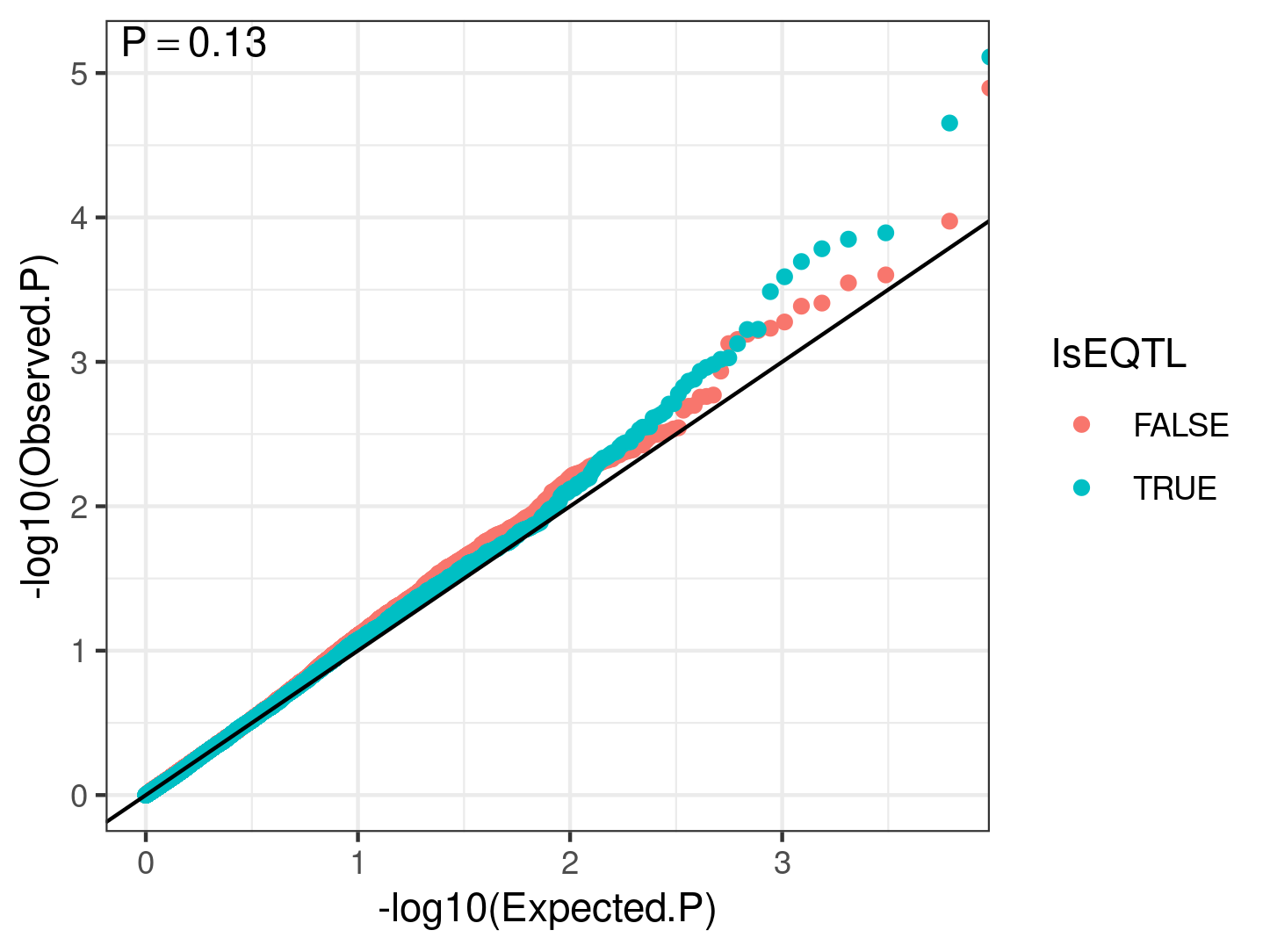
I checked if eQTL SNPs (top SNPs for GTEX heart left ventricle eGenes (FDR<0.01) ) have generally smaller P-values than a same sized random sample of non eQTL SNPs, using a QQ-plot:
 .
.
My interpretation of this is that eQTLs generally are not driven by cell type QTLs. Another thing I could ask is if the top cell type QTLs (some which may be false positives), are closer to highly dispersed genes compared to lowly dispersed genes.
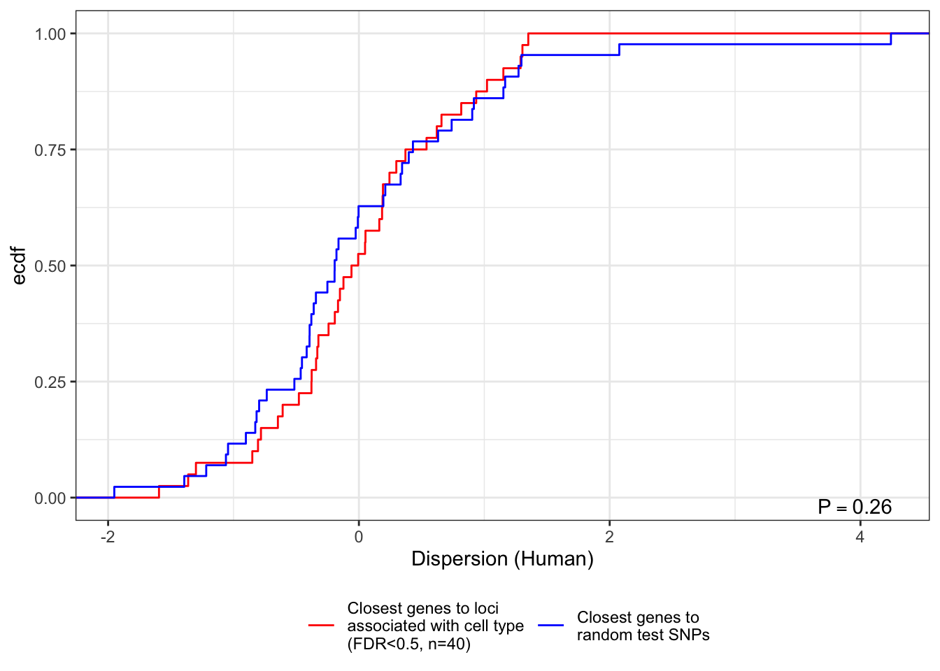
Despite no SNPs exceeding standard GWAS significance (P<5E-8) I have taken the 98 most significant loci (lumped by clustering into the best SNP within 250000 of any locus than contains a SNP with FDR (Storey’s Q) less than 0.5) and found the closest gene for which I estimated dispersion (SNPs further than 100kb from any of these genes were discarded). I have done the same for a set of random test SNPs for comparison.
Let’s plot the dispersion for these closest gene SNPs, with the closest genes to the random control SNPs as a comparison.
library(tidyverse)

GWAS.Snps <- read.table("../output/CellProportionGWAS.RandomControlloci.closestGenes.txt", sep = ' ', col.names = c("gene", "dist"))
Control.Snps <- read.table("../output/CellProportionGWAS.Testloci.closestGenes.txt", sep = ' ', col.names = c("gene", "dist"))

AllClosestGenes <- dplyr::bind_rows(list(CellTypeAssociatedSNPs=GWAS.Snps, RandomTestSNPs=Control.Snps), .id = 'source') %>%
  mutate(gene=str_remove(gene, "\\.\\d+$"))
head(AllClosestGenes)
source gene dist
1 CellTypeAssociatedSNPs ENSG00000171960 78877
2 CellTypeAssociatedSNPs ENSG00000066557 61156
3 CellTypeAssociatedSNPs ENSG00000138185 8280
4 CellTypeAssociatedSNPs ENSG00000095587 63564
5 CellTypeAssociatedSNPs ENSG00000188385 55631
6 CellTypeAssociatedSNPs ENSG00000175356 65094Dispersion <- read.delim('../output/OverdispersionEstimatesFromChimp.txt')
TestResults <-AllClosestGenes %>%
left_join(Dispersion, by="gene") %>%
wilcox.test(Human.Residual~source, data=., alternative="greater")
TestResults
    Wilcoxon rank sum test

data:  Human.Residual by source
W = 932, p-value = 0.2583
alternative hypothesis: true location shift is greater than 0
lb1 = paste0('P==', format.pval(TestResults$p.value, 2))
AllClosestGenes %>%
left_join(Dispersion, by="gene") %>%
ggplot(aes(x=Human.Residual, color=source)) +
stat_ecdf() +
xlab("Dispersion (Human)") +
ylab("ecdf") +
annotate("text",x=Inf,y=-Inf, label=lb1, hjust=1.5, vjust=-0.5, parse=TRUE) +
scale_color_manual(name=NULL, values=c("red", "blue"), labels=c("Closest genes to loci\nassociated with cell type\n(FDR<0.5, n=40)", "Closest genes to\nrandom test SNPs")) +
theme_bw() +
theme(legend.position="bottom")
And write out the plot…
ggsave("../figures/OriginalArt/ResponseToReviewers.GWAS.ClosestGenes.pdf", height=3, width=3.65)
sessionInfo()R version 3.6.1 (2019-07-05)
Platform: x86_64-apple-darwin15.6.0 (64-bit)
Running under: macOS Catalina 10.15.5
Matrix products: default
BLAS: /Library/Frameworks/R.framework/Versions/3.6/Resources/lib/libRblas.0.dylib
LAPACK: /Library/Frameworks/R.framework/Versions/3.6/Resources/lib/libRlapack.dylib
locale:
[1] en_US.UTF-8/en_US.UTF-8/en_US.UTF-8/C/en_US.UTF-8/en_US.UTF-8
attached base packages:
[1] stats graphics grDevices utils datasets methods base
other attached packages:
[1] forcats_0.4.0 stringr_1.4.0 dplyr_0.8.3 purrr_0.3.3
[5] readr_1.3.1 tidyr_1.0.0 tibble_2.1.3 ggplot2_3.2.1
[9] tidyverse_1.3.0
loaded via a namespace (and not attached):
[1] tidyselect_0.2.5 xfun_0.11 haven_2.2.0 lattice_0.20-38
[5] colorspace_1.4-1 vctrs_0.2.0 generics_0.0.2 htmltools_0.4.0
[9] yaml_2.2.0 rlang_0.4.1 later_1.0.0 pillar_1.4.2
[13] withr_2.1.2 glue_1.3.1 DBI_1.0.0 dbplyr_1.4.2
[17] modelr_0.1.5 readxl_1.3.1 lifecycle_0.1.0 munsell_0.5.0
[21] gtable_0.3.0 workflowr_1.5.0 cellranger_1.1.0 rvest_0.3.5
[25] evaluate_0.14 labeling_0.3 knitr_1.26 httpuv_1.5.2
[29] fansi_0.4.0 broom_0.5.2 Rcpp_1.0.5 promises_1.1.0
[33] backports_1.1.5 scales_1.1.0 jsonlite_1.6 farver_2.0.1
[37] fs_1.3.1 hms_0.5.2 digest_0.6.23 stringi_1.4.3
[41] grid_3.6.1 rprojroot_1.3-2 cli_2.0.0 tools_3.6.1
[45] magrittr_1.5 lazyeval_0.2.2 crayon_1.3.4 whisker_0.4
[49] pkgconfig_2.0.3 zeallot_0.1.0 xml2_1.2.2 reprex_0.3.0
[53] lubridate_1.7.4 rstudioapi_0.10 assertthat_0.2.1 rmarkdown_1.18
[57] httr_1.4.1 R6_2.4.1 nlme_3.1-143 git2r_0.26.1
[61] compiler_3.6.1