ResponseToReviewer_Point6

workflowr

• Summary
• Checks
• Past versions

Last updated: 2020-09-23

Checks: 6 1

Knit directory: Comparative_eQTL/analysis/

This reproducible R Markdown analysis was created with workflowr (version 1.5.0). The Checks tab describes the reproducibility checks that were applied when the results were created. The Past versions tab lists the development history.

---

R Markdown file: uncommitted changes

The R Markdown file has unstaged changes. To know which version of the R Markdown file created these results, you’ll want to first commit it to the Git repo. If you’re still working on the analysis, you can ignore this warning. When you’re finished, you can run wflow_publish to commit the R Markdown file and build the HTML.

Environment: empty

Great job! The global environment was empty. Objects defined in the global environment can affect the analysis in your R Markdown file in unknown ways. For reproduciblity it’s best to always run the code in an empty environment.

Seed: set.seed(20190319)

The command set.seed(20190319) was run prior to running the code in the R Markdown file. Setting a seed ensures that any results that rely on randomness, e.g. subsampling or permutations, are reproducible.

Session information: recorded

Great job! Recording the operating system, R version, and package versions is critical for reproducibility.

Cache: none

Nice! There were no cached chunks for this analysis, so you can be confident that you successfully produced the results during this run.

File paths: relative

Great job! Using relative paths to the files within your workflowr project makes it easier to run your code on other machines.

Repository version: 52f85bb

Great! You are using Git for version control. Tracking code development and connecting the code version to the results is critical for reproducibility. The version displayed above was the version of the Git repository at the time these results were generated.

Note that you need to be careful to ensure that all relevant files for the analysis have been committed to Git prior to generating the results (you can use wflow_publish or wflow_git_commit). workflowr only checks the R Markdown file, but you know if there are other scripts or data files that it depends on. Below is the status of the Git repository when the results were generated:

Ignored files:
    Ignored:    .DS_Store
    Ignored:    .RData
    Ignored:    .Rhistory
    Ignored:    .Rproj.user/
    Ignored:    WorkingManuscript.zip
    Ignored:    WorkingManuscript/
    Ignored:    analysis/.DS_Store
    Ignored:    analysis/.Rhistory
    Ignored:    analysis_temp/.DS_Store
    Ignored:    big_data/
    Ignored:    code/.DS_Store
    Ignored:    code/snakemake_workflow/.DS_Store
    Ignored:    code/snakemake_workflow/.Rhistory
    Ignored:    data/.DS_Store
    Ignored:    data/PastAnalysesDataToKeep/.DS_Store
    Ignored:    figures/
    Ignored:    output/.DS_Store

Untracked files:
    Untracked:  analysis/20200907_Response_Point_02.Rmd
    Untracked:  analysis/20200907_Response_Point_04.Rmd
    Untracked:  data/c5.all.v7.1.symbols.gmt
    Untracked:  data/c5.all.v7.1.symbols.gmt.categories.tsv.gz
    Untracked:  data/h.all.v7.1.symbols.gmt

Unstaged changes:
    Modified:   analysis/20200907_Response_OriginalComments.Rmd
    Modified:   analysis/20200907_Response_Point_06.Rmd
    Modified:   analysis/20200907_Response_Point_09-2.Rmd
    Modified:   analysis/20200907_Response_Point_09.Rmd
    Modified:   analysis/20200907_Response_Point_11.Rmd
    Modified:   analysis/Final_2_DispersionPlots.Rmd
    Modified:   analysis_temp/TabulaMuris_analysis2.Rmd

Note that any generated files, e.g. HTML, png, CSS, etc., are not included in this status report because it is ok for generated content to have uncommitted changes.

---

These are the previous versions of the R Markdown and HTML files. If you’ve configured a remote Git repository (see ?wflow_git_remote), click on the hyperlinks in the table below to view them.

File	Version	Author	Date	Message
Rmd	25874ad	Benjmain Fair	2020-09-10	update site
html	25874ad	Benjmain Fair	2020-09-10	update site
Rmd	5f95cbc	Benjmain Fair	2020-09-10	update site
html	5f95cbc	Benjmain Fair	2020-09-10	update site

---

Original reviewer point:

I would like to see more discussion about the inter-relatedness of the chimpanzees in the analysis of gene expression. Is that contributing to the power of the DE analysis, which has really high numbers of DE genes. That may certainly be due to the large samples size, but should be addressed. Related to that, the support that the gene-wise dispersion estimates are well correlated in humans and chimpanzees overall (Fig1C, and S4) seems qualitative. It looks like the chimpanzees might have less dispersion overall?

I will address the first point (about relatedness in DE analysis) two ways. Firstly, I will use variance partition to argue that the relatedness of some of the chimps probably has little impact on the interspecies DE analysis, given that a relatively much larger fraction of variance will probably be explained species, batch, etc. Then I will empricially address this by reperforming DE analysis with subsamples of chimps that have some relatively high degree of inter-relatedness, compared to subsamples that do not have such relatedness.

First load necessary libraries for analysis…

library(tidyverse)
library(gplots)
library(readxl)
library(scales)
library(variancePartition)
library('limma')
library('edgeR')
library(pbapply)
library(knitr)
library(readxl)

source("../code/CustomFunctions.R")

Load relatedness matrix and RNA-seq sample batch info

#Relatedness matrix
SampleLabels <- read.table('../output/ForAssociationTesting.temp.fam', stringsAsFactors = F)$V2
GemmaMatrix <- as.matrix(read.table('../output/GRM.cXX.txt'))
colnames(GemmaMatrix) <- SampleLabels
row.names(GemmaMatrix) <- SampleLabels

#Metadata like RNA-seq batch
Metadata<-read_excel("../data/Metadata_SequencedChimps.xlsx")
Metadata$RNA.Extract_date %>% unique() %>% length()

[1] 5

Metadata$RNA.Library.prep.batch %>% unique() %>% length()

[1] 5

Colors <- data.frame(Numbers=1:5, Colors=hue_pal()(5))

BatchColor <- data.frame(IndividualID=as.character(colnames(GemmaMatrix))) %>% 
  left_join(Metadata, by=c("IndividualID"="IndividualID (as listed in vcf)")) %>%
  dplyr::select(IndividualID, RNA.Library.prep.batch) %>%
  left_join(Colors, by=c("RNA.Library.prep.batch"="Numbers")) %>%
  pull(Colors) %>% as.character()

diag(GemmaMatrix) <- NA #For plotting purposes, just don't show the diagonol so that the color scale is better for non-diagnol entries

hclustfunc <- function(x) hclust(x, method="complete")
distfunc <- function(x) dist(x,method="euclidean")
d <- distfunc(GemmaMatrix)
fit <- hclustfunc(d)
groups <- cutree(fit, k=7) 

NumbersToColors <- function(NumberVector){
  N <- length(unique(NumberVector))
  Key <- setNames(hue_pal()(N), 1:N)
  return(list(ColorVector=recode(NumberVector, !!!Key), Key=Key))
}

ClusterGroupColors <- NumbersToColors(groups)

heatmap.2(GemmaMatrix, trace="none", RowSideColors = ClusterGroupColors$ColorVector, ColSideColors = BatchColor)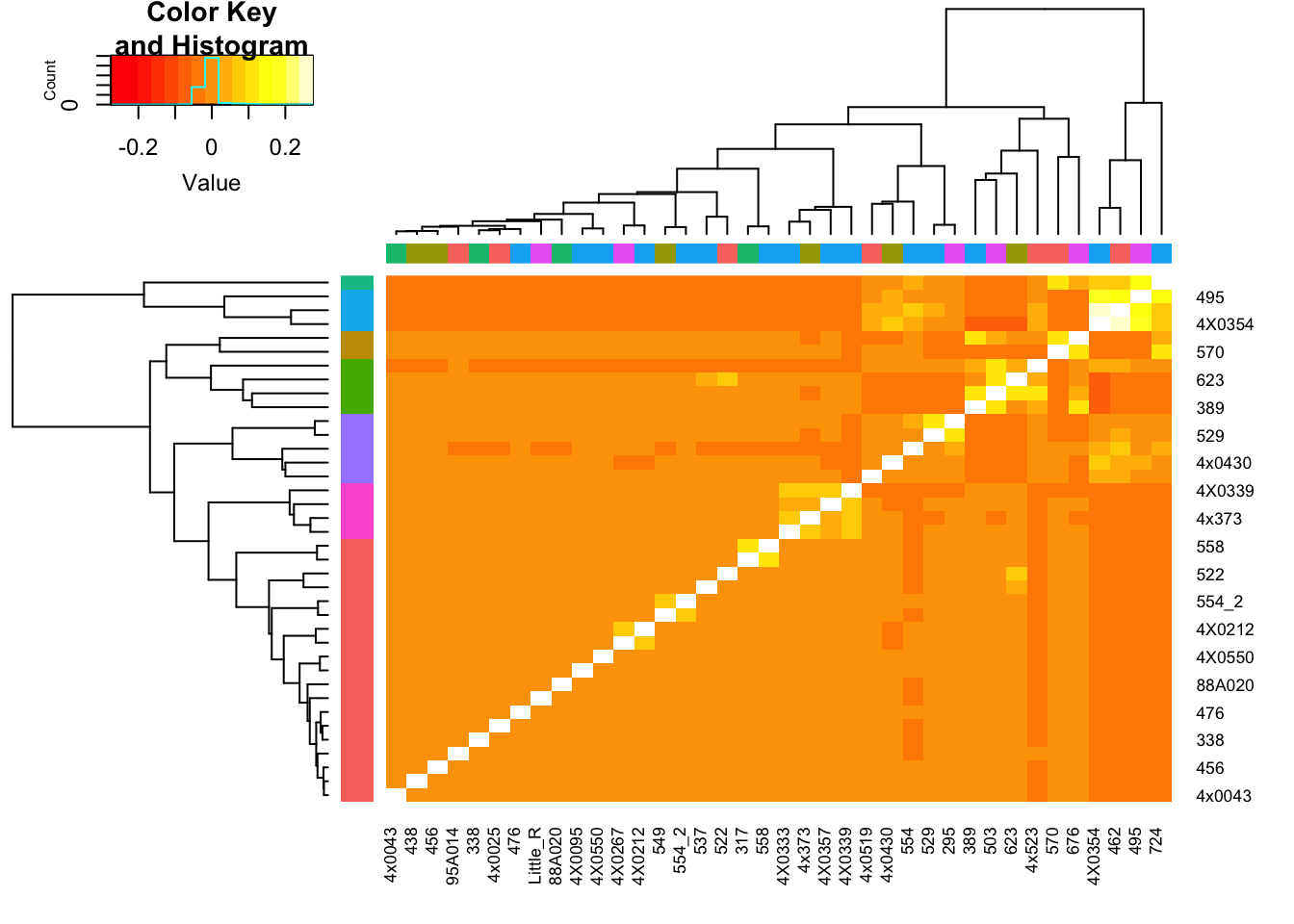

Past versions of unnamed-chunk-2-1.png

Version	Author	Date
25874ad	Benjmain Fair	2020-09-10
5f95cbc	Benjmain Fair	2020-09-10

Column colors are RNA library prep batch, row colors are cluster groups (cutree function). I may pick out some of those somewhat related sample blocks for DE analysis…

Groups.df<-as.data.frame(groups) %>% rownames_to_column("Ind")

GemmaMatrix %>% as.data.frame() %>%
  rownames_to_column("IndA") %>%
  gather(key="IndB", value="Kinship", -IndA) %>%
  left_join(Groups.df, by=c("IndA"="Ind")) %>%
  left_join(Groups.df, by=c("IndB"="Ind"), suffix=c(".A.group", ".B.group")) %>%
  filter(groups.A.group==groups.B.group & !IndA==IndB) %>%
  mutate(uniqueID = paste0(pmax(IndA, IndB), pmin(IndA, IndB))) %>%
  distinct(uniqueID, .keep_all=T) %>%
  mutate(groups.A.group=factor(groups.A.group)) %>%
  ggplot(aes(x=groups.A.group, y=Kinship, color=groups.A.group)) +
  geom_boxplot(outlier.shape = NA) +
  geom_jitter(position=position_jitter(0.2)) +
  ylab("Pairwise kinship coefficients within cluster") +
  xlab("Cluster") +
  scale_colour_manual(name = "ClusterGroup",values = ClusterGroupColors$Key) +
  theme_bw() +
  theme(legend.position = "none")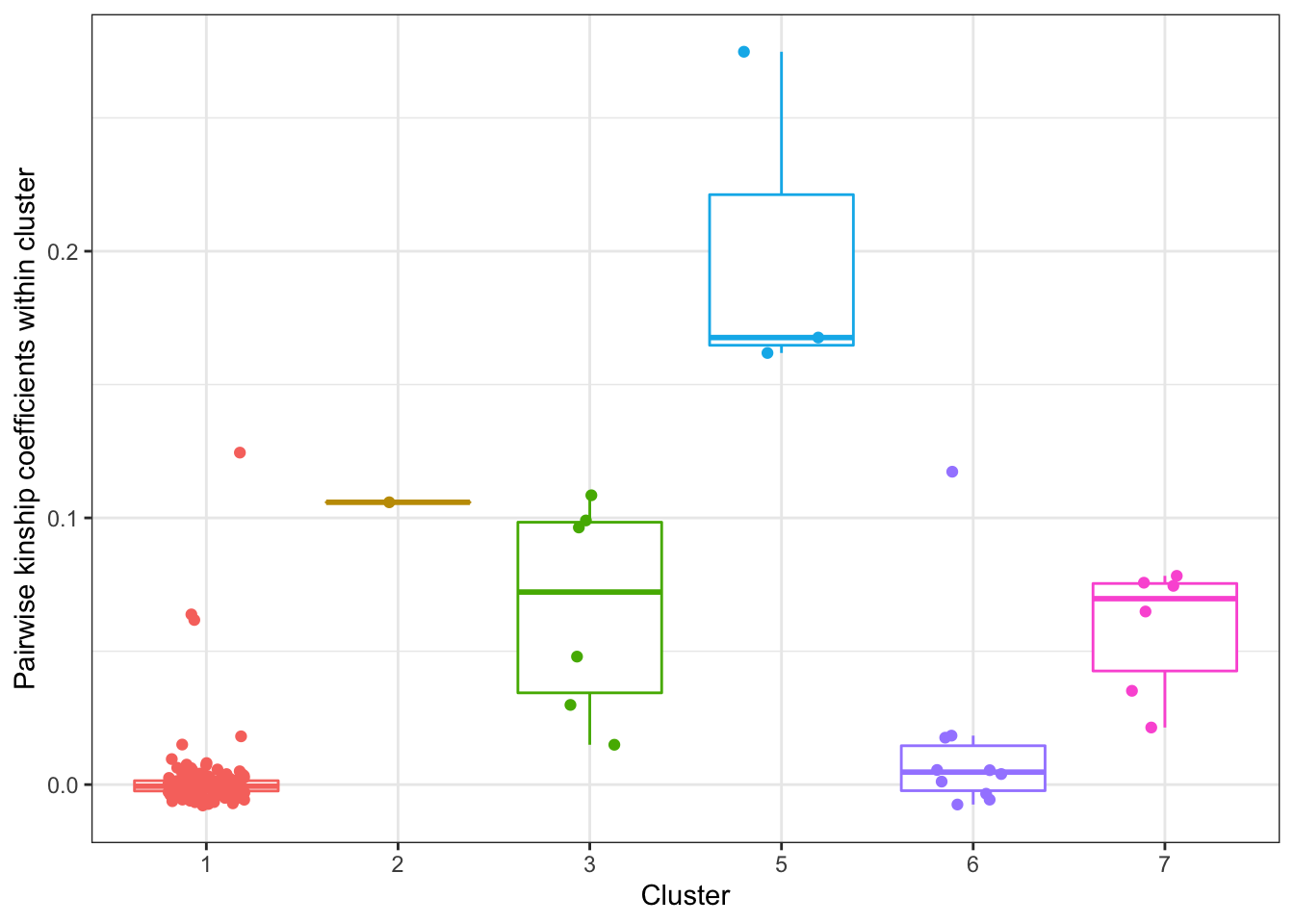

Now let’s select samples from cluster 1,3,6,7, and perform DE analysis using only 4 samples (4Chimp + 4Human) from each cluster and compare. If relatedness plays a big (meaningful) role, I expect meaningful differences in the the number of DE genes, the fraction of false discoveries, etc. Since clusters 3, and 7 only have 4 or 5 samples, I will use all 4 samples from these clusters. For cluster6, I will exclude the least related sample (smallest average pairwase intra-cluster relatedness). For cluster1, since there are so many samples, most of which have small relatedness coefficients, I exclude the 6 samples with a relatedness coefficient > 0.05, (leaving all unrelated samples) and randomly draw (with replacement) subsamples of 4 for DE analysis, repeating this procedure many times to establish a null distribution to compare clusters 3,6 & 7.

#First, create a dataframe containing only the samples that will be considered for further analysis as described above.
#Show cluster identities:
Groups.df %>% head() %>% kable()

Ind	groups
549	1
570	2
389	3
456	1
623	3
438	1

#Get the 4 samples to include for cluster3
Cluster3.Pool <- Groups.df %>% filter(groups==3) %>% pull(Ind)

#Get the 4 samples to include for cluster7
Cluster7.Pool <- Groups.df %>% filter(groups==7) %>% pull(Ind)

#Get samples to include from cluster6
#I want to include 4/5 in that cluster, excluding the sample with lowest mean pairwise kinship.
CLuster6.MeanpairwiseKinship <- GemmaMatrix %>% as.data.frame() %>%
  rownames_to_column("IndA") %>%
  gather(key="IndB", value="Kinship", -IndA) %>%
  left_join(Groups.df, by=c("IndA"="Ind")) %>%
  left_join(Groups.df, by=c("IndB"="Ind"), suffix=c(".A.group", ".B.group")) %>%
  distinct(uniqueID, .keep_all=T) %>%
  filter(groups.A.group==6 & groups.B.group==6 & !IndA==IndB) %>%
  group_by(IndA) %>%
  summarize(MeanPairwiseKinship=mean(Kinship))
kable(CLuster6.MeanpairwiseKinship)

IndA	MeanPairwiseKinship
295	0.0338598
4x0430	-0.0009190
4x0519	0.0017661
529	0.0310048
554	0.0106422

Cluster6.Pool <- CLuster6.MeanpairwiseKinship %>%
  filter(MeanPairwiseKinship>min(MeanPairwiseKinship)) %>% pull(IndA)

#Get cluster1 pool. I want to include all samples in cluter1 that do not have any related individuals (kinship coefficients > 0.05)
CLuster1.MaxpairwiseKinship <- GemmaMatrix %>% as.data.frame() %>%
  rownames_to_column("IndA") %>%
  gather(key="IndB", value="Kinship", -IndA) %>%
  left_join(Groups.df, by=c("IndA"="Ind")) %>%
  left_join(Groups.df, by=c("IndB"="Ind"), suffix=c(".A.group", ".B.group")) %>%
  distinct(uniqueID, .keep_all=T) %>%
  filter(groups.A.group==1 & groups.B.group==1 & !IndA==IndB) %>%
  group_by(IndA) %>%
  summarize(MaxPairwiseKinship=max(Kinship))
kable(CLuster1.MaxpairwiseKinship)

IndA	MaxPairwiseKinship
317	0.1244824
338	0.0068539
438	0.0080694
456	0.0095653
476	0.0072819
4x0025	0.0072819
4x0043	0.0095653
4X0095	0.0150108
4X0212	0.0617353
4X0267	0.0617353
4X0550	0.0150108
522	0.0180964
537	0.0052832
549	0.0638122
554_2	0.0638122
558	0.1244824
88A020	0.0026078
95A014	0.0049990
Little_R	0.0180964

Cluster1.Pool <- CLuster1.MaxpairwiseKinship %>%
  filter(MaxPairwiseKinship<0.05) %>% pull(IndA)

SamplesToDrawFrom <- cbind(Cluster1.Pool, Cluster3.Pool, Cluster6.Pool, Cluster7.Pool) %>%
  as.data.frame() %>%
  gather(key="Cluster", "Ind") %>%
  distinct(.keep_all=T)

SamplesToDrawFrom %>% kable()

Cluster	Ind
Cluster1.Pool	338
Cluster1.Pool	438
Cluster1.Pool	456
Cluster1.Pool	476
Cluster1.Pool	4x0025
Cluster1.Pool	4x0043
Cluster1.Pool	4X0095
Cluster1.Pool	4X0550
Cluster1.Pool	522
Cluster1.Pool	537
Cluster1.Pool	88A020
Cluster1.Pool	95A014
Cluster1.Pool	Little_R
Cluster3.Pool	389
Cluster3.Pool	623
Cluster3.Pool	503
Cluster3.Pool	4x523
Cluster6.Pool	295
Cluster6.Pool	4x0519
Cluster6.Pool	529
Cluster6.Pool	554
Cluster7.Pool	4x373
Cluster7.Pool	4X0333
Cluster7.Pool	4X0357
Cluster7.Pool	4X0339

Ok. So now I have pools of samples to draw from for clusters 1,3,6,7.

I will do one DE analysis for clusters 3,6,7, and many analyses for cluster1 to establish a null distribution of no relatedness. I think for this question it makes sense to make the repeated analysis with random from cluster1 sampling without replacement. So there are \(13 nCr 4 = 715\) possible combinations of samples to create this null distribution. That is a small enough number I will just do all of them to establish as rich of a null as possible.

But first, let’s choose the human samples to compare to for this DE analysis. I think there is no point in introducing randomness to the human samples drawn. But I think it does make sense to carefully choose them to be as high quality as possible, for example, by controlling for batch/lab. Therefore, I think I should use 4 human sampleschosen from Pavlovic et al in my DE analysis. Let’s pick these randomly.

ColColors <- ClusterGroupColors$ColorVector
ColColors[!(rownames(GemmaMatrix) %in% SamplesToDrawFrom$Ind)] <- NA
heatmap.2(GemmaMatrix, trace="none", RowSideColors = ClusterGroupColors$ColorVector, ColSideColors = ColColors)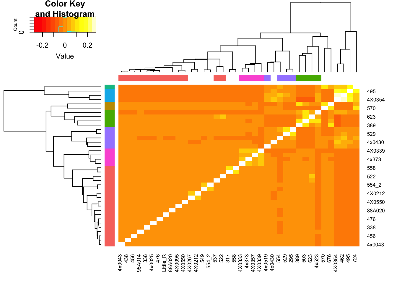

PairwiseKinshipBoxplot <- GemmaMatrix %>% as.data.frame() %>%
  rownames_to_column("IndA") %>%
  gather(key="IndB", value="Kinship", -IndA) %>%
  left_join(Groups.df, by=c("IndA"="Ind")) %>%
  left_join(Groups.df, by=c("IndB"="Ind"), suffix=c(".A.group", ".B.group")) %>%
  filter(groups.A.group==groups.B.group & !IndA==IndB) %>%
  filter(IndA %in% SamplesToDrawFrom$Ind & IndB %in% SamplesToDrawFrom$Ind ) %>%
  mutate(uniqueID = paste0(pmax(IndA, IndB), pmin(IndA, IndB))) %>%
  distinct(uniqueID, .keep_all=T) %>%
  mutate(groups.A.group=factor(groups.A.group)) %>%
  ggplot(aes(x=groups.A.group, y=Kinship, color=groups.A.group)) +
  geom_boxplot(outlier.shape = NA) +
  geom_jitter(position=position_jitter(0.2)) +
  ylab("Pairwise kinship coefficients\nwithin cluster") +
  xlab("Filtered kinship cluster") +
  scale_colour_manual(name = "ClusterGroup",values = ClusterGroupColors$Key) +
  theme_bw() +
  theme(legend.position = "none", axis.text.x=element_blank())
PairwiseKinshipBoxplot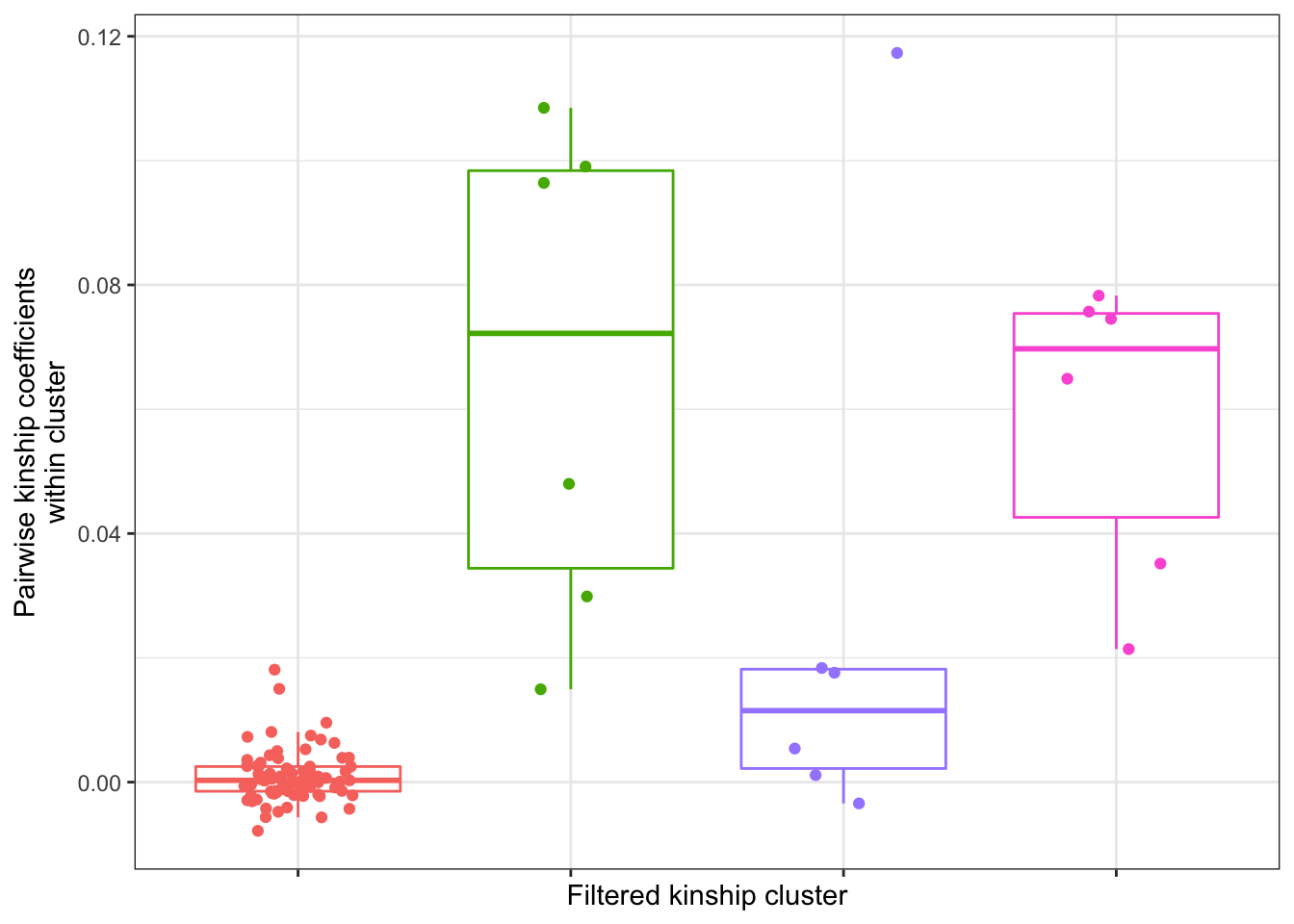

Now let’s wrap the desired DE analysis into a function for easier repitition:

###Define function
DE.analysis <- function(DGE.NormalizedRawCountTable, Log2RPKMCountTable, ChimpSamples, HumanSamples){
  AllSamplesToSubset <- c(ChimpSamples, HumanSamples)
  CountTableSampled <- DGE.NormalizedRawCountTable[,AllSamplesToSubset]
  SpeciesFactor <- colnames(CountTableSampled) %>% substr(1,1) %>% factor() %>% unclass() %>% as.character()
  mm <- model.matrix(~0 + SpeciesFactor)
  y <- voom(CountTableSampled, mm, normalize.method="cyclicloess", plot=F)
  y$E <- Log2RPKMCountTable[,AllSamplesToSubset]
  
  fit<- lmFit(y, mm)
  contr <- makeContrasts(DE=SpeciesFactor1-SpeciesFactor2, levels = mm)
  tmp <- contrasts.fit(fit, contrasts=contr)
  efit <- eBayes(tmp)
  Results <- topTable(efit, sort.by = "none", n=Inf)
  return(Results)
}

###Create some of the required arguments

CountTableChimpFile <- '../output/PowerAnalysisFullCountTable.Chimp.subread.txt.gz'
CountTableHumanFile <- '../output/PowerAnalysisFullCountTable.Human.subread.txt.gz'
OutputDE <- '../output/Final/TableS2.tab'
DropFileName <- '../data/DE_SamplesToDrop.txt'

DropFile <- read.delim(DropFileName, sep='\t', col.names = c("Sample", "Species"), stringsAsFactors = F)
HumanSamplesToDrop <- DropFile %>% filter(Species=="Human") %>% pull(Sample)
ChimpSamplesToDrop <- DropFile %>% filter(Species=="Chimp") %>% pull(Sample)
DE.results <- read.delim(OutputDE, sep='\t', stringsAsFactors = F)
GeneListForOverdispersionCalculation <- DE.results$Ensembl_geneID

CountTables <- GetCountTables(CountTableChimpFile,
                              CountTableHumanFile,
                              0, GeneListForOverdispersionCalculation, ChimpSampleDrop=ChimpSamplesToDrop, HumanSampleDrop = HumanSamplesToDrop)

DGE.NormalizedRawCountTable <- cbind(CountTables$Chimp$Counts, CountTables$Human$Counts )
  DGEList() %>%
  calcNormFactors()

An object of class "DGEList"
$counts
<0 x 0 matrix>

$samples
[1] group        lib.size     norm.factors
<0 rows> (or 0-length row.names)

Log2RPKMCountTable <- cbind(CountTables$Chimp$log2RPKM, CountTables$Human$log2RPKM)

set.seed(0)
HumanSamples <- colnames(CountTables$Human$Counts)[CountTables$Human$Counts %>% colnames() %>% str_detect("SRR", negate = T)] %>%
  sample(4)
ChimpSamples <- paste0("C.", Cluster3.Pool)


###print the required arguments to illustrate what is going on
DGE.NormalizedRawCountTable[1:10,1:10] %>% kable()

C	.4x0519 C	.4x373 C	.476 C	.4x0025 C	.438 C	.462 C	.4X0354 C	.503 C	.317 C	.623
ENSG00000186891	46	73	20	28	4	11	98	13	11	3
ENSG00000186827	274	393	313	397	173	128	975	236	307	84
ENSG00000078808	5967	1931	7637	3892	2957	3745	1189	5857	4306	3704
ENSG00000176022	1097	402	1574	1333	955	1235	416	1087	745	640
ENSG00000184163	7	49	113	62	62	29	111	82	24	18
ENSG00000160087	761	283	1153	776	471	610	275	920	547	604
ENSG00000162572	7	4	17	2	5	16	12	11	9	10
ENSG00000131584	2587	1537	3646	2546	1755	1323	4585	2250	1484	1872
ENSG00000169972	282	78	396	257	209	282	111	243	141	252
ENSG00000127054	3009	2009	7404	3300	3600	2092	3147	4403	2740	3116

Log2RPKMCountTable[1:10,1:10] %>% kable()

	C.4x0519	C.4x373	C.476	C.4x0025	C.438	C.462	C.4X0354	C.503	C.317	C.623
ENSG00000186891	-0.4631141	1.5452701	-1.7906428	-0.7436310	-2.7486168	-2.037643	1.502654	-1.8335368	-1.867155	-3.0690602
ENSG00000186827	1.8312433	3.7552296	1.7373802	2.7719656	1.9481646	1.020653	4.595932	1.8981157	2.472714	0.8400153
ENSG00000078808	4.9992002	4.7877280	5.0681744	4.7966794	4.7681080	4.602012	3.621035	5.2552587	5.012015	5.0089176
ENSG00000176022	3.0009070	2.9687688	3.2341574	3.6942616	3.5811589	3.445338	2.551394	3.2700042	2.926360	2.9213715
ENSG00000184163	-3.1250345	0.5876174	0.1042405	-0.0550313	0.3005269	-1.218992	1.285548	0.2081517	-1.277634	-1.4597615
ENSG00000160087	2.3164984	2.3055132	2.6277490	2.7569100	2.4056076	2.272207	1.798519	2.8713177	2.323592	2.6794380
ENSG00000162572	-4.2857112	-3.8425882	-3.5385672	-5.0822034	-4.0764170	-3.142342	-2.918254	-3.5855126	-3.656867	-3.3581316
ENSG00000131584	3.2105543	3.8747917	3.4183582	3.6009371	3.4321338	2.518798	4.982773	3.2921295	2.892687	3.4412337
ENSG00000169972	2.2566182	1.8242974	2.4572966	2.5336727	2.6025630	2.528399	1.864482	2.3241553	1.747091	2.7869341
ENSG00000127054	4.0532149	4.8857942	5.0644684	4.5997661	5.0927794	3.803711	5.064977	4.8847706	4.401255	4.8006463

HumanSamples

[1] "H.63145" "H.62606" "H.59167" "H.59263"

ChimpSamples

[1] "C.389"   "C.623"   "C.503"   "C.4x523"

###Test the function
Results <- DE.analysis(DGE.NormalizedRawCountTable=DGE.NormalizedRawCountTable, ChimpSamples=ChimpSamples, Log2RPKMCountTable=Log2RPKMCountTable, HumanSamples=HumanSamples)
Results %>% head() %>% kable()

	logFC	AveExpr	t	P.Value a	dj.P.Val	B
ENSG00000186891	1.1813874	-1.6752344	1.130220	0.2869894	0.4529246	-5.551883
ENSG00000186827	-1.2248842	2.5200273	-2.274735	0.0483767	0.1449773	-4.895913
ENSG00000078808	0.2885241	5.0609380	1.559132	0.1526664	0.3005444	-6.245397
ENSG00000176022	0.1927662	3.0497948	1.255078	0.2403959	0.4041648	-6.572526
ENSG00000184163	-0.7863931	0.0711966	-1.606493	0.1418966	0.2868254	-5.390743
ENSG00000160087	0.3136660	2.5227387	1.724462	0.1179827	0.2542184	-5.893499

Ok, so I have a function to do the DE analysis. Let’s use it to compare all combinations of the Cluster1.Pool of chimp samples vs 4 human samples, and do a similar analysis but with the cluster3Pool, cluster6Pool, and cluster7Pool.

#First get all combinations of samples in cluster1Pool.

Cluster1.Combinations <- combn(Cluster1.Pool, 4, simplify = F)
Cluster1.Combinations.Pasted <- lapply(Cluster1.Combinations, function(iter) paste0("C.", iter))
length(Cluster1.Combinations.Pasted)

[1] 715

Cluster1.Combinations.Pasted[1:10]

[[1]]
[1] "C.338" "C.438" "C.456" "C.476"

[[2]]
[1] "C.338"    "C.438"    "C.456"    "C.4x0025"

[[3]]
[1] "C.338"    "C.438"    "C.456"    "C.4x0043"

[[4]]
[1] "C.338"    "C.438"    "C.456"    "C.4X0095"

[[5]]
[1] "C.338"    "C.438"    "C.456"    "C.4X0550"

[[6]]
[1] "C.338" "C.438" "C.456" "C.522"

[[7]]
[1] "C.338" "C.438" "C.456" "C.537"

[[8]]
[1] "C.338"    "C.438"    "C.456"    "C.88A020"

[[9]]
[1] "C.338"    "C.438"    "C.456"    "C.95A014"

[[10]]
[1] "C.338"      "C.438"      "C.456"      "C.Little_R"

Note that since this takes a long time to compute the DE results for 715 combinations, I will turn this code block to eval=F and write out the results, and read in the results in the next code block…

#iterate over combinations list, and calculate DE results for each
Cluster1.Combinations.Results <-pbapply::pblapply(Cluster1.Combinations.Pasted, function(iter) DE.analysis(HumanSamples=HumanSamples, Log2RPKMCountTable=Log2RPKMCountTable, DGE.NormalizedRawCountTable=DGE.NormalizedRawCountTable, ChimpSamples = iter))


#Write out results
saveRDS(Cluster1.Combinations.Results, file = "../big_data/Cluster1_DE_Results_AllCombinations.rds")

Let’s start by plotting the number of DE genes (at a few FDR thresholds) when each of the clusters 3, 6, and 7 were used for the chimp samples, and compare it to the distribution across all 715 combinations from cluster 1.

#Read in results
Cluster1.Combinations.Results <- readRDS("../big_data/Cluster1_DE_Results_AllCombinations.rds")

Cluster1.Combinations.Results.df <- Cluster1.Combinations.Results %>%
  lapply(add_rownames, "Ensembl_geneID") %>%
  bind_rows(.id="CombinationNumber")

#DE analysis for other cluster groups
OtherClusters.df <- SamplesToDrawFrom %>% filter(!Cluster=="Cluster1.Pool") %>%
  mutate(Ind=paste0("C.", Ind))
OtherClusters.list <- split(OtherClusters.df$Ind, OtherClusters.df$Cluster)

OtherClusters.Results <-pbapply::pblapply(OtherClusters.list, function(iter) DE.analysis(HumanSamples=HumanSamples, Log2RPKMCountTable=Log2RPKMCountTable, DGE.NormalizedRawCountTable=DGE.NormalizedRawCountTable, ChimpSamples = iter))

OtherClusters.Results.df <- OtherClusters.Results %>%
  lapply(add_rownames, "Ensembl_geneID") %>%
  bind_rows(.id="ClusterNumber") %>%
  mutate(ClusterNumber=gsub("Cluster(\\d).Pool", "\\1", ClusterNumber))
  

NumResults <- OtherClusters.Results.df %>%
  dplyr::select(adj.P.Val, ClusterNumber) %>%
  mutate(FDR.10 = adj.P.Val < 0.10,
         FDR.05 = adj.P.Val < 0.05,
         FDR.01 = adj.P.Val < 0.01,) %>%
  gather(key="FDR", value="Signif", -adj.P.Val, -ClusterNumber) %>%
  group_by(ClusterNumber, FDR) %>%
  summarise(NumSigGenes=sum(Signif))


ToPlotNumSig <- Cluster1.Combinations.Results.df %>%
  dplyr::select(adj.P.Val, CombinationNumber) %>%
  mutate(FDR.10 = adj.P.Val < 0.10,
         FDR.05 = adj.P.Val < 0.05,
         FDR.01 = adj.P.Val < 0.01,) %>%
  gather(key="FDR", value="Signif", -adj.P.Val, -CombinationNumber) %>%
  group_by(CombinationNumber, FDR) %>%
  summarise(NumSigGenes=sum(Signif)) %>%
  mutate(Cluster1.Combinations="1")

NumDE.Plot <- ggplot(ToPlotNumSig, aes(x=NumSigGenes)) +
  # stat_ecdf(color=ClusterGroupColors$Key[1]) +
  geom_density(aes(fill=Cluster1.Combinations)) +
  geom_vline(data=NumResults, size=1, aes(xintercept=NumSigGenes, color=ClusterNumber)) +
  facet_wrap(~FDR, scales="free_y") +
  ylab("empirical probability density") +
  xlab("Num DE genes") +
  scale_colour_manual(name = "Cluster",values = ClusterGroupColors$Key, labels=NULL) +
  scale_fill_manual(name = "All nCr(13,4)=715\ncombinations",values = ClusterGroupColors$Key, labels=NULL) +
  theme_bw() +
  theme(axis.text.x = element_text(angle = 45))

NumDE.Plot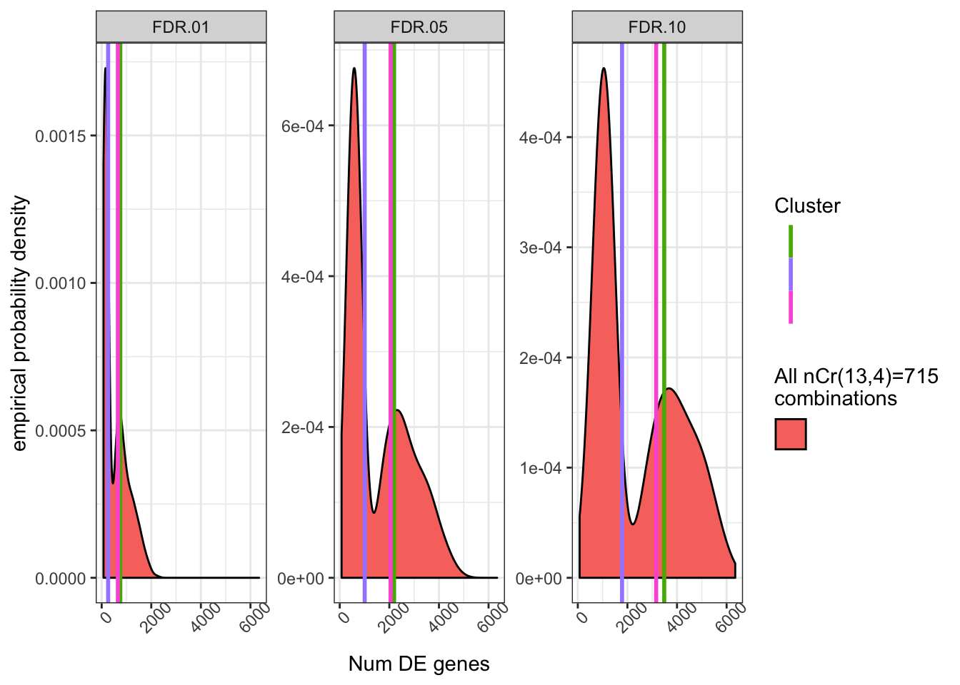

The bimodal distribution is a bit odd, and probably reflects two or three “bad” samples in the group of 13 samples in cluster13 which skew results to less genes when randomly drawn. I suppose odd things are expected when randomly drawing from such a small sample size. In any case, I think we are fundamentally limited towards fully emperically quantifying the relatedness effect reviewers comment. But in any case, it doesn’t seem like there is any drastic effect.

Let’s make similar plots but plotting the empirical FDR (based on FDR<0.01 genes from the full data set as the ad hoc gold standard).

ToPlotFDR <- Cluster1.Combinations.Results.df %>%
  dplyr::select(adj.P.Val, CombinationNumber, Ensembl_geneID) %>%
  mutate(FDR.10 = adj.P.Val < 0.10,
         FDR.05 = adj.P.Val < 0.05,
         FDR.01 = adj.P.Val < 0.01) %>%
  dplyr::select(FDR.10:FDR.01, CombinationNumber, Ensembl_geneID) %>%
  gather(key="FDR", value="Signif", -CombinationNumber, -Ensembl_geneID) %>%
  left_join(DE.results, by="Ensembl_geneID") %>%
  mutate(TrueResponse = adj.P.Val < 0.01) %>%
  mutate(CorrectResponse = (TrueResponse & Signif)) %>%
  group_by(CombinationNumber, FDR) %>%
  summarise(NumSigGenes=1-sum(CorrectResponse)/sum(Signif)) %>%
  mutate(Cluster1.Combinations="1")


FDR.Results <- OtherClusters.Results.df %>%
  dplyr::select(adj.P.Val, ClusterNumber, Ensembl_geneID) %>%
  mutate(FDR.10 = adj.P.Val < 0.10,
         FDR.05 = adj.P.Val < 0.05,
         FDR.01 = adj.P.Val < 0.01) %>%
  dplyr::select(FDR.10:FDR.01, ClusterNumber, Ensembl_geneID) %>%
  gather(key="FDR", value="Signif", -ClusterNumber, -Ensembl_geneID) %>%
  left_join(DE.results, by="Ensembl_geneID") %>%
  mutate(TrueResponse = adj.P.Val < 0.01) %>%
  mutate(CorrectResponse = (TrueResponse & Signif)) %>%
  group_by(ClusterNumber, FDR) %>%
  summarise(NumSigGenes=1-sum(CorrectResponse)/sum(Signif))

FDR.Plot <- ggplot(ToPlotFDR, aes(x=NumSigGenes)) +
  # stat_ecdf(color=ClusterGroupColors$Key[1]) +
  geom_density(aes(fill=Cluster1.Combinations)) +
  geom_vline(data=FDR.Results, size=1, aes(xintercept=NumSigGenes, color=ClusterNumber)) +
  facet_wrap(~FDR, scales="free_y") +
  ylab("empirical probability density") +
  xlab("Empirical FDR estimate") +
  scale_colour_manual(name = "Cluster",values = ClusterGroupColors$Key, labels=NULL) +
  scale_fill_manual(name = "All nCr(13,4)=715\ncombinations",values = ClusterGroupColors$Key, labels=NULL) +
  theme_bw() +
  theme(axis.text.x = element_text(angle = 45))
FDR.Plot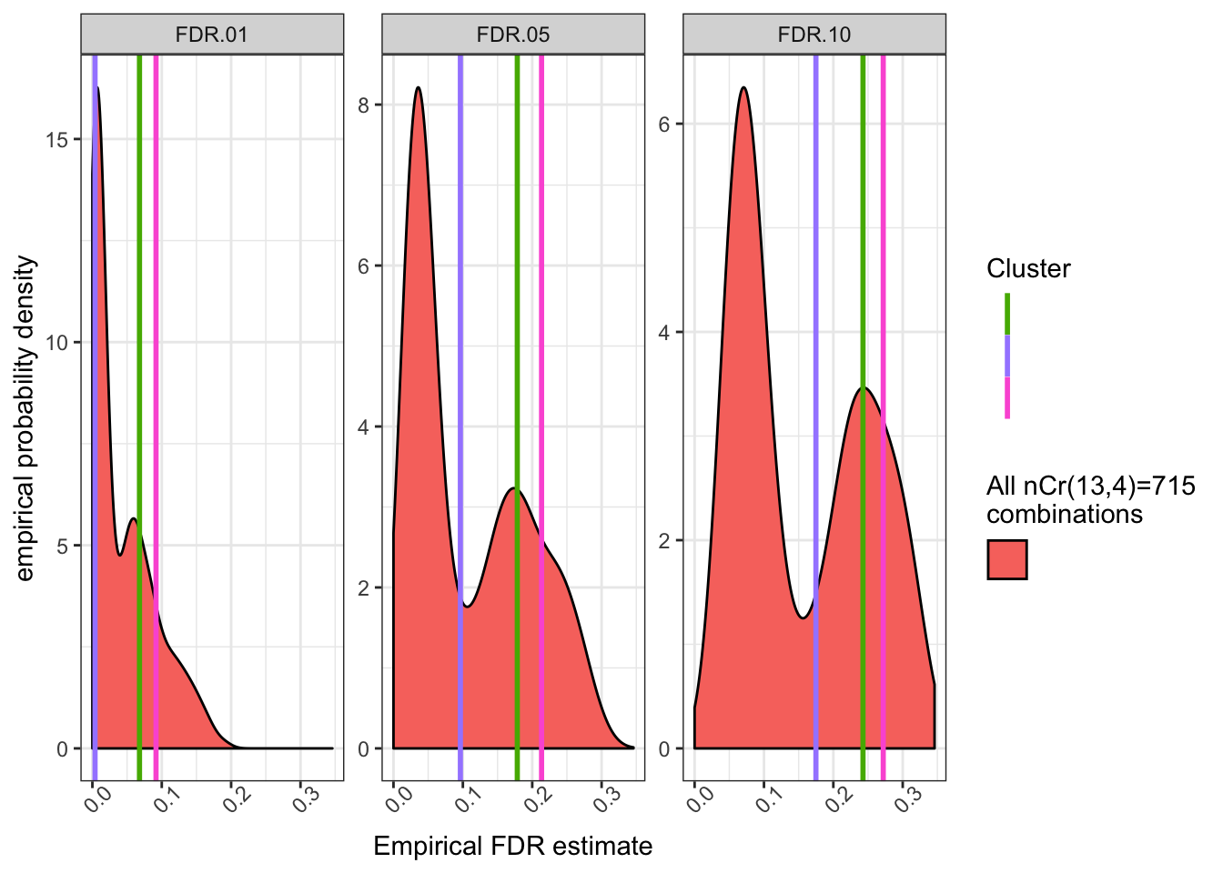

Now let’s try to explain that bimodal shape in the cluster1 combinations… Let’s start by looking at a PCA or hiearchal clustering of the cluster1 samples to look for outliers, and see if the inclusion of such outliers in the combinations is causing the bimodal shape.

Cluster1.CountTable <- CountTables$Chimp$log2RPKM %>%
  dplyr::select(one_of(
    paste0("C.", SamplesToDrawFrom %>% filter(Cluster=="Cluster1.Pool") %>% pull(Ind))
  ))

PCA <- Cluster1.CountTable %>%
  t() %>% prcomp()

Metadata <- read.delim("../output/Final/TableS1.tab", stringsAsFactors = F) %>%
  dplyr::select(IID=Sample.ID, SX, SP, UniquelyMappingReads, RNA.Extraction.Batch, RIN, PercentUniquelyMappingReads) %>%
  mutate(IID=paste0("C.", IID))

PCA$x %>% as.data.frame() %>% dplyr::select(PC1:PC2) %>%
  rownames_to_column("IID") %>%
  left_join(Metadata, by="IID") %>%
  ggplot(aes(x=PC1, y=PC2, color=PercentUniquelyMappingReads)) +
  geom_text(aes(label=IID)) +
  theme_bw()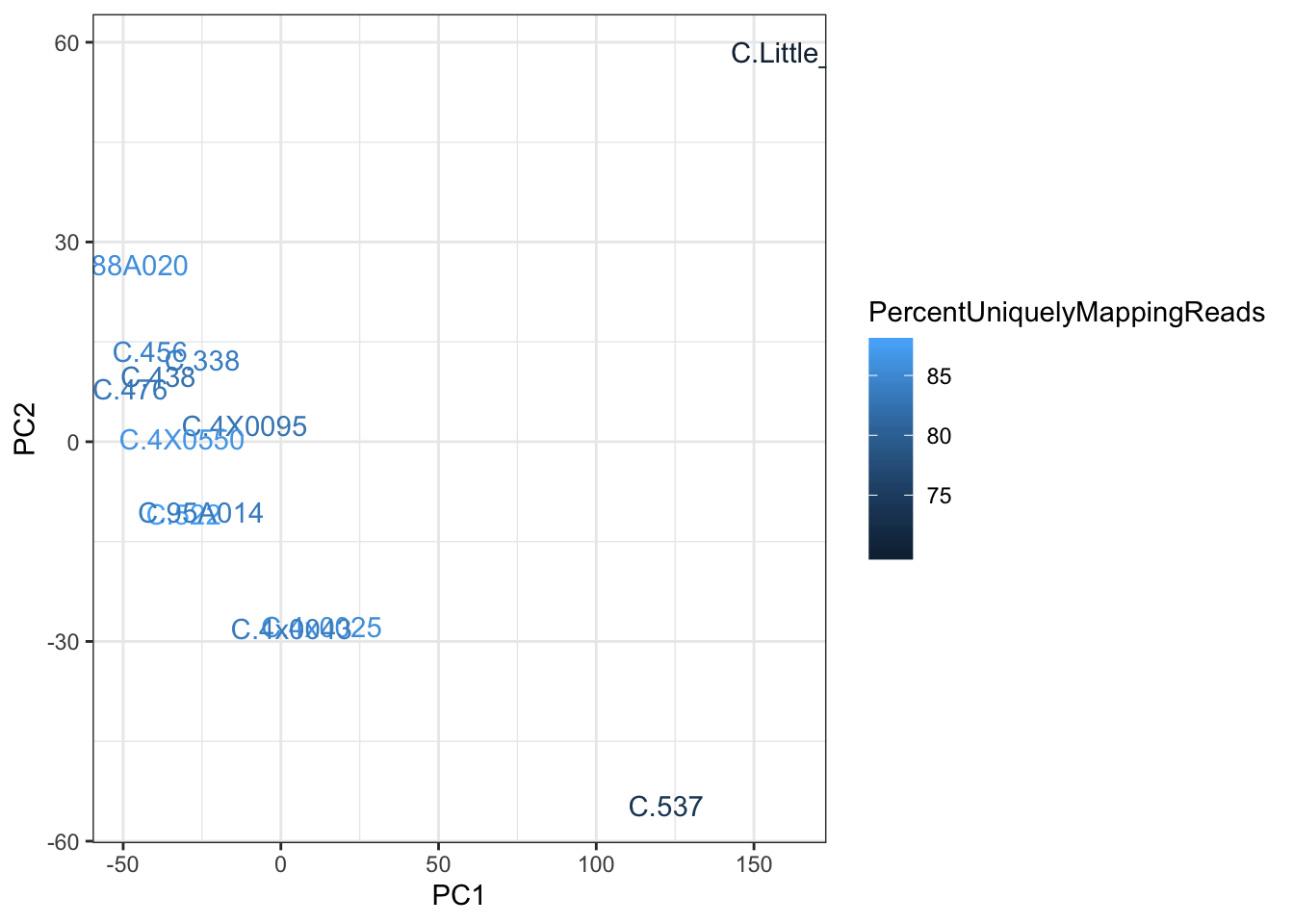

Cluster1.CountTable %>% cor() %>%
  heatmap.2()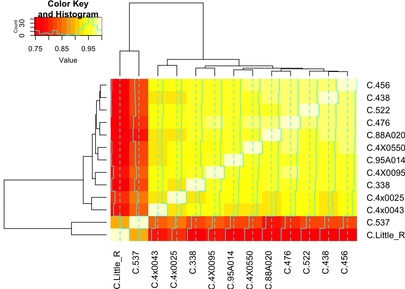

CountTables$Chimp$log2RPKM %>%
  dplyr::select(one_of(
    paste0("C.", SamplesToDrawFrom %>% pull(Ind))
  )) %>% cor() %>%
  heatmap.2()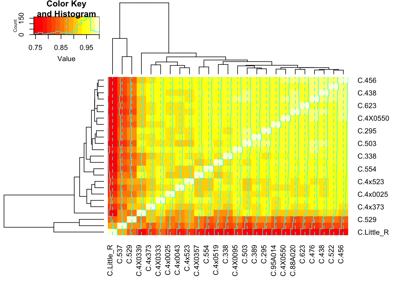

There are indeed two outliers. Let’s see if those are responsible for the bimodal shape…

ClusterOneCombinationsWithOutliers <- Cluster1.Combinations.Pasted %>%
  unlist() %>%
  matrix(byrow=T, nrow=length(Cluster1.Combinations.Pasted)) %>%
  as.data.frame() %>%
  mutate(CombinationNumber=1:n(),
         CombinationPasted=paste(V1,V2,V3,V4)) %>%
  mutate(ContainsOutliers=str_detect(CombinationPasted, "C.Little_R|C.537")) %>%
  filter(ContainsOutliers==T) %>%
  pull(CombinationNumber)


ToPlotNumSig %>%
  mutate(ContainsOutliers=CombinationNumber %in% ClusterOneCombinationsWithOutliers) %>%
ggplot(aes(x=NumSigGenes)) +
  # stat_ecdf(color=ClusterGroupColors$Key[1]) +
  geom_density(aes(fill=Cluster1.Combinations, linetype=ContainsOutliers)) +
  geom_vline(data=NumResults, size=1, aes(xintercept=NumSigGenes, color=ClusterNumber)) +
  facet_wrap(~FDR, scales="free_y") +
  ylab("empirical probability density") +
  xlab("Num DE genes") +
  scale_colour_manual(name = "Cluster",values = ClusterGroupColors$Key, labels=NULL) +
  scale_fill_manual(name = "All nCr(13,4)=715\ncombinations",values = ClusterGroupColors$Key, labels=NULL) +
  theme_bw() +
  theme(axis.text.x = element_text(angle = 45))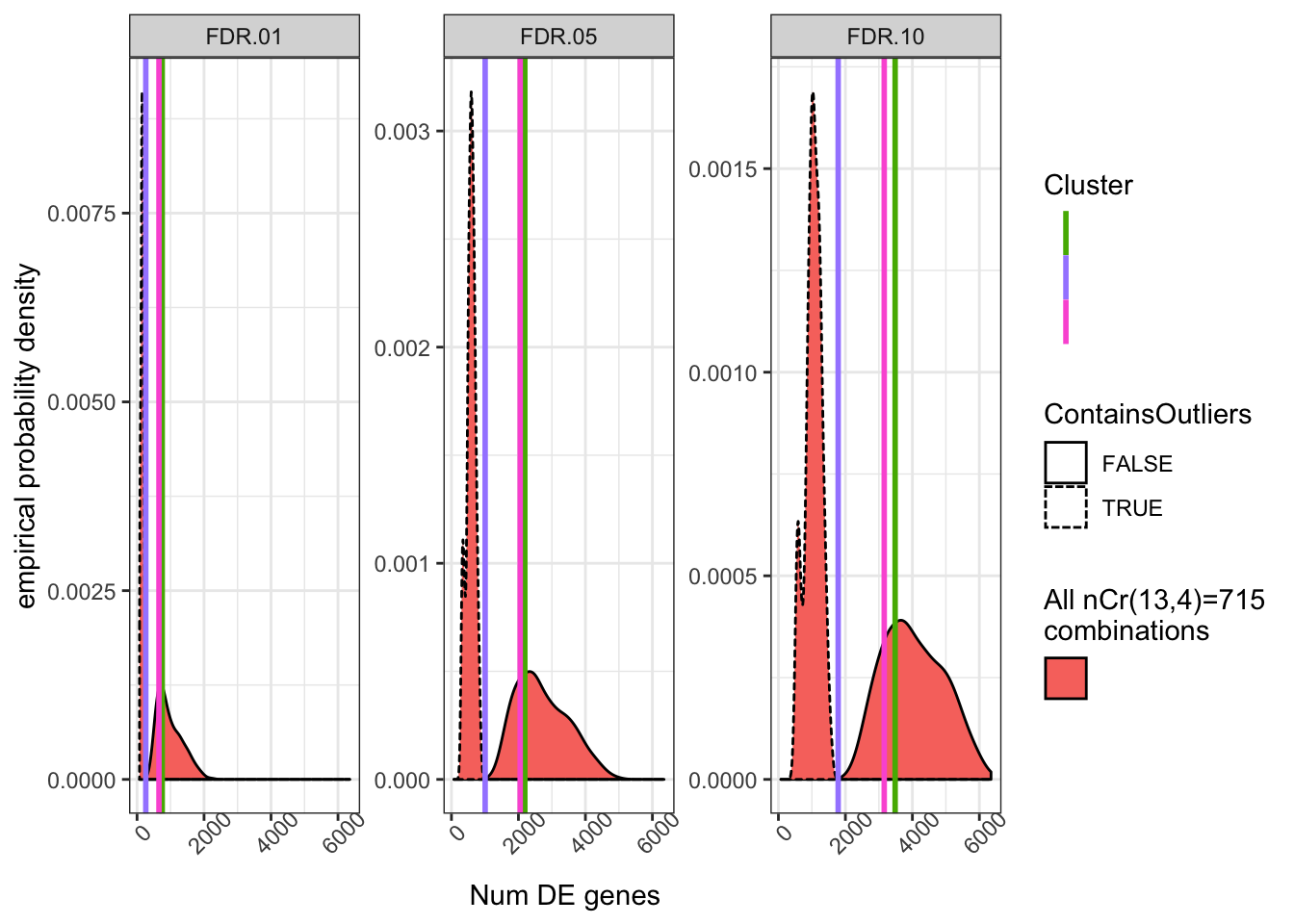

Ok. I think I want to just remake some of the previous plots, but show how these outliers have a different distribution.

Start with a heatmap of RNA-seq data from all the samples included in this analysis, colored by group, and batch.

I’m going to set this code block to eval=F so that it doesn’t take as long to build this html doc.

CorMatToPlot <- CountTables$Chimp$log2RPKM %>%
  dplyr::select(one_of(
    paste0("C.", SamplesToDrawFrom %>% pull(Ind))
  )) %>% cor()

MetadataForHeatMap <- data.frame(C.Ind=rownames(CorMatToPlot)) %>%
  mutate(Ind=str_remove(C.Ind, "^C.")) %>%
  left_join(SamplesToDrawFrom, by ="Ind") %>%
  mutate(ClusterNumber=gsub("Cluster(\\d).Pool", "\\1", Cluster)) %>%
  left_join(data.frame(Color=ClusterGroupColors$Key) %>% rownames_to_column("ClusterNumber"), by="ClusterNumber") %>%
  left_join(Metadata %>% dplyr::select(RNA.Extraction.Batch, IID), by=c("C.Ind"="IID"))


rownames(CorMatToPlot) <- str_remove(rownames(CorMatToPlot), "^C.")
colnames(CorMatToPlot) <- str_remove(colnames(CorMatToPlot), "^C.")

pdf(file="../figures/OriginalArt/ResponseToReviewers.DE.ExpressionMat.pdf")
heatmap.2(CorMatToPlot, trace="none", RowSideColors = MetadataForHeatMap$RNA.Extraction.Batch %>% as.factor() %>% as.numeric() %>% as.character(), ColSideColors = MetadataForHeatMap$Color %>% as.character(), dendrogram="row")
dev.off()


pdf(file="../figures/OriginalArt/ResponseToReviewers.DE.KinshipMat.pdf")
heatmap.2(GemmaMatrix, trace="none", RowSideColors = ClusterGroupColors$ColorVector, ColSideColors = ColColors, dendrogram="row")
dev.off()

NumDE.Plot <- ToPlotNumSig %>%
  mutate(ContainsOutliers=CombinationNumber %in% ClusterOneCombinationsWithOutliers) %>%
ggplot(aes(x=NumSigGenes)) +
  # stat_ecdf(color=ClusterGroupColors$Key[1]) +
  geom_density(aes(fill=Cluster1.Combinations, linetype=ContainsOutliers), alpha=0.9) +
  geom_vline(data=NumResults, size=1, aes(xintercept=NumSigGenes, color=ClusterNumber)) +
  facet_wrap(~FDR, scales="free_y") +
  ylab("empirical density") +
  xlab("Num DE genes") +
  scale_colour_manual(name = "Filtered\nkinship clusters", values = ClusterGroupColors$Key, labels=NULL) +
  scale_fill_manual(name = "All nCr(13,4)=715\ncombinations",values = ClusterGroupColors$Key, labels=NULL) +
  scale_linetype_manual(name="Combinations that contain samples\n'Little_R' or '537'", values=c("solid", "dashed")) +
  theme_bw() +
  theme(axis.text.x = element_text(angle = 45), legend.position = "bottom") +
    guides(color = guide_legend(title.position = "top"),
         linetype = guide_legend(title.position = "top"),
         fill = guide_legend(title.position = "top"))
NumDE.Plot

FDR.Plot <- ToPlotFDR %>%
  mutate(ContainsOutliers=CombinationNumber %in% ClusterOneCombinationsWithOutliers) %>%
  ggplot(aes(x=NumSigGenes)) +
  # stat_ecdf(color=ClusterGroupColors$Key[1]) +
  geom_density(aes(x=NumSigGenes, ..density.., fill=Cluster1.Combinations, linetype=ContainsOutliers), alpha=0.9) +
  geom_vline(data=FDR.Results, size=1, aes(xintercept=NumSigGenes, color=ClusterNumber)) +
  facet_wrap(~FDR, scales="free_y") +
  ylab("empirical density") +
  xlab("Empirical FDR estimate") +
  scale_colour_manual(name = "Filtered\nkinship clusters",values = ClusterGroupColors$Key, labels=NULL) +
  scale_fill_manual(name = "All nCr(13,4)=715\ncombinations",values = ClusterGroupColors$Key, labels=NULL) +
  scale_linetype_manual(name="Combinations that contain samples\n'Little_R' or '537'", values=c("solid", "dashed")) +
  theme_bw() +
  theme(axis.text.x = element_text(angle = 45), legend.position = "bottom") +
  guides(color = guide_legend(title.position = "top"),
         linetype = guide_legend(title.position = "top"),
         fill = guide_legend(title.position = "top"))
FDR.Plot


ggsave("../figures/OriginalArt/ResponseToReviewers.DE.PairwiseKinship.pdf", plot=PairwiseKinshipBoxplot, height=3, width=2.5)
ggsave("../figures/OriginalArt/ResponseToReviewers.DE.NumDE.pdf", plot=NumDE.Plot, height=3, width=6.5)
ggsave("../figures/OriginalArt/ResponseToReviewers.DE.FDR.pdf", plot=FDR.Plot, height=3, width=6.5)

Also, let’s use the variance partition to describe how much gene expression variance (among the chimp samples only) can be explained by factors like sex, batch, RIN, and the kinship cluster groups. Also turning eval=F because variance partition takes a few minutes. But the figures generated will be published in the paper or as part of the public response to reviewers.

info <- read.delim("../output/Final/TableS1.tab", stringsAsFactors = F) %>%
  dplyr::select(Alternate.ID, IID=Sample.ID, SX, SP, UniquelyMappingReads, RNA.Extraction.Batch, RIN, PercentUniquelyMappingReads) %>%
  mutate(SP=recode(SP, Human="H", Chimp="C")) %>%
  filter(SP=="C") %>%
  inner_join(Groups.df, by=c("IID"="Ind")) %>%
  mutate(Individual=paste0("C.", IID))

gExpr <- cbind(CountTables$Chimp$Counts) %>%
  dplyr::select(one_of(info$Individual)) %>%
  DGEList() %>%
  calcNormFactors
vobjGenes <- voom(gExpr)

info <- info %>%
  filter(Individual %in% colnames(gExpr)) %>%
  column_to_rownames("Individual")


form <- ~  RIN + SX + RNA.Extraction.Batch + groups

varPart <- fitExtractVarPartModel( vobjGenes, form, info )

# sort variables (i.e. columns) by median fraction # of variance explained
vp <- sortCols( varPart )

# violin plot of contribution of each variable to total variance
plotVarPart( vp )



info <- read_excel("../data/Metadata_SequencedChimps.xlsx") %>%
  dplyr::select(IID=1, SX, RNA.Extraction.Batch=RNA.Extract_date, RNA.Library.prep.batch, RIN) %>%
  mutate(RNA.Library.prep.batch=as.factor(RNA.Library.prep.batch)) %>%
  # inner_join(Groups.df, by=c("IID"="Ind")) %>%
  inner_join(SamplesToDrawFrom, by=c("IID"="Ind")) %>%
  dplyr::rename(groups=Cluster) %>%
  mutate(groups=as.factor(groups)) %>%
  mutate(Individual=paste0("C.", IID))
gExpr <- cbind(CountTables$Chimp$Counts) %>%
  dplyr::select(one_of(info$Individual)) %>%
  DGEList() %>%
  calcNormFactors
vobjGenes <- voom(gExpr)

info <- info %>%
  filter(Individual %in% colnames(gExpr)) %>%
  column_to_rownames("Individual")


# form <- ~  RIN + (1|SX) + (1|RNA.Extraction.Batch)  + (1|groups)
# varPart <- fitExtractVarPartModel( vobjGenes, form, info )

form <- ~  (1|SX) + (1|RNA.Extraction.Batch)  + (1|groups)
varPart <- fitExtractVarPartModel( vobjGenes, form, info )


# sort variables (i.e. columns) by median fraction # of variance explained
vp <- sortCols( varPart )

# violin plot of contribution of each variable to total variance
VarPartPlot <- plotVarPart( vp ) +
  scale_x_discrete(labels=c("SX" = "Sex", "groups"="Filtered\nkinship clusters"))

f <- function(x) {
  r <- quantile(x, probs = c(0.05, 0.25, 0.5, 0.75, 0.95))
  names(r) <- c("ymin", "lower", "middle", "upper", "ymax")
  r
}

VarPartPlot <- vp %>%
  gather(key="factor", value="Variance explained (%)") %>%
  ggplot(aes(x=fct_reorder(factor, `Variance explained (%)`), y=`Variance explained (%)`)) +
  stat_summary(fun.data=f, geom="boxplot") + 
  scale_x_discrete(labels=c("SX" = "Sex", "groups"="Filtered\nkinship clusters")) +
  xlab("") +
  theme_bw() +
  theme(axis.text.x = element_text(angle = 45, hjust = 1))


ggsave("../figures/OriginalArt/ResponseToReviewers.DE.KinshipVarPart.pdf", VarPartPlot, height=3.5, width=2.5)

Session information

sessionInfo()

R version 3.6.1 (2019-07-05)
Platform: x86_64-apple-darwin15.6.0 (64-bit)
Running under: macOS Catalina 10.15.5

Matrix products: default
BLAS:   /Library/Frameworks/R.framework/Versions/3.6/Resources/lib/libRblas.0.dylib
LAPACK: /Library/Frameworks/R.framework/Versions/3.6/Resources/lib/libRlapack.dylib

locale:
[1] en_US.UTF-8/en_US.UTF-8/en_US.UTF-8/C/en_US.UTF-8/en_US.UTF-8

attached base packages:
[1] parallel  stats     graphics  grDevices utils     datasets  methods  
[8] base     

other attached packages:
 [1] cowplot_1.0.0            gridExtra_2.3            MASS_7.3-51.4           
 [4] knitr_1.26               pbapply_1.4-3            edgeR_3.26.8            
 [7] variancePartition_1.14.1 Biobase_2.44.0           BiocGenerics_0.30.0     
[10] foreach_1.4.7            limma_3.40.6             scales_1.1.0            
[13] readxl_1.3.1             gplots_3.0.1.1           forcats_0.4.0           
[16] stringr_1.4.0            dplyr_0.8.3              purrr_0.3.3             
[19] readr_1.3.1              tidyr_1.0.0              tibble_2.1.3            
[22] ggplot2_3.2.1            tidyverse_1.3.0         

loaded via a namespace (and not attached):
 [1] nlme_3.1-143        bitops_1.0-6        fs_1.3.1           
 [4] pbkrtest_0.4-8.6    lubridate_1.7.4     doParallel_1.0.15  
 [7] progress_1.2.2      httr_1.4.1          rprojroot_1.3-2    
[10] tools_3.6.1         backports_1.1.5     R6_2.4.1           
[13] KernSmooth_2.23-16  DBI_1.0.0           lazyeval_0.2.2     
[16] colorspace_1.4-1    withr_2.1.2         prettyunits_1.0.2  
[19] tidyselect_0.2.5    compiler_3.6.1      git2r_0.26.1       
[22] cli_2.0.0           rvest_0.3.5         xml2_1.2.2         
[25] labeling_0.3        caTools_1.17.1.3    digest_0.6.23      
[28] minqa_1.2.4         rmarkdown_1.18      colorRamps_2.3     
[31] pkgconfig_2.0.3     htmltools_0.4.0     lme4_1.1-23        
[34] highr_0.8           dbplyr_1.4.2        rlang_0.4.1        
[37] rstudioapi_0.10     farver_2.0.1        generics_0.0.2     
[40] jsonlite_1.6        BiocParallel_1.18.1 gtools_3.8.1       
[43] magrittr_1.5        Matrix_1.2-18       Rcpp_1.0.5         
[46] munsell_0.5.0       fansi_0.4.0         lifecycle_0.1.0    
[49] stringi_1.4.3       whisker_0.4         yaml_2.2.0         
[52] plyr_1.8.5          grid_3.6.1          gdata_2.18.0       
[55] promises_1.1.0      crayon_1.3.4        lattice_0.20-38    
[58] haven_2.2.0         splines_3.6.1       hms_0.5.2          
[61] locfit_1.5-9.1      zeallot_0.1.0       pillar_1.4.2       
[64] boot_1.3-23         reshape2_1.4.3      codetools_0.2-16   
[67] reprex_0.3.0        glue_1.3.1          evaluate_0.14      
[70] modelr_0.1.5        vctrs_0.2.0         nloptr_1.2.2.2     
[73] httpuv_1.5.2        cellranger_1.1.0    gtable_0.3.0       
[76] assertthat_0.2.1    xfun_0.11           broom_0.5.2        
[79] later_1.0.0         iterators_1.0.12    workflowr_1.5.0    
[82] statmod_1.4.34      ellipsis_0.3.0