2024-01-17_CheckYangsJunctionAnnotator

workflowr

• Summary
• Checks
• Past versions

Last updated: 2024-06-06

Checks: 5 2

Knit directory: ChromatinSplicingQTLs/analysis/

This reproducible R Markdown analysis was created with workflowr (version 1.7.0). The Checks tab describes the reproducibility checks that were applied when the results were created. The Past versions tab lists the development history.

---

R Markdown file: uncommitted changes

The R Markdown file has unstaged changes. To know which version of the R Markdown file created these results, you’ll want to first commit it to the Git repo. If you’re still working on the analysis, you can ignore this warning. When you’re finished, you can run wflow_publish to commit the R Markdown file and build the HTML.

Environment: empty

Great job! The global environment was empty. Objects defined in the global environment can affect the analysis in your R Markdown file in unknown ways. For reproduciblity it’s best to always run the code in an empty environment.

Seed: set.seed(20191126)

The command set.seed(20191126) was run prior to running the code in the R Markdown file. Setting a seed ensures that any results that rely on randomness, e.g. subsampling or permutations, are reproducible.

Session information: recorded

Great job! Recording the operating system, R version, and package versions is critical for reproducibility.

Cache: none

Nice! There were no cached chunks for this analysis, so you can be confident that you successfully produced the results during this run.

File paths: absolute

Using absolute paths to the files within your workflowr project makes it difficult for you and others to run your code on a different machine. Change the absolute path(s) below to the suggested relative path(s) to make your code more reproducible.

absolute	relative
/project2/yangili1/bjf79/ChromatinSplicingQTLs/data/igsr_samples.tsv.gz	../data/igsr_samples.tsv.gz

Repository version: 209c2d5

Great! You are using Git for version control. Tracking code development and connecting the code version to the results is critical for reproducibility.

The results in this page were generated with repository version 209c2d5. See the Past versions tab to see a history of the changes made to the R Markdown and HTML files.

Note that you need to be careful to ensure that all relevant files for the analysis have been committed to Git prior to generating the results (you can use wflow_publish or wflow_git_commit). workflowr only checks the R Markdown file, but you know if there are other scripts or data files that it depends on. Below is the status of the Git repository when the results were generated:

Ignored files:
    Ignored:    .DS_Store
    Ignored:    .Rhistory
    Ignored:    .Rproj.user/
    Ignored:    analysis/.Rhistory
    Ignored:    code/.DS_Store
    Ignored:    code/.RData
    Ignored:    code/._report.html
    Ignored:    code/.ipynb_checkpoints/
    Ignored:    code/.snakemake/
    Ignored:    code/APA_Processing/
    Ignored:    code/Alignments/
    Ignored:    code/ChromHMM/
    Ignored:    code/ENCODE/
    Ignored:    code/ExpressionAnalysis/
    Ignored:    code/ExtractPhenotypeBedByGenotype.py
    Ignored:    code/FastqFastp/
    Ignored:    code/FastqFastpSE/
    Ignored:    code/FastqSE/
    Ignored:    code/FineMapping/
    Ignored:    code/GTEx/
    Ignored:    code/Gencode.v34.6Colors.bed.gz
    Ignored:    code/Genotypes/
    Ignored:    code/H3K36me3_CutAndTag.pdf
    Ignored:    code/IntronSlopes/
    Ignored:    code/LR.bed
    Ignored:    code/LR.seq.bed
    Ignored:    code/LongReads/
    Ignored:    code/MYB.tracks.ini
    Ignored:    code/Metaplots/
    Ignored:    code/Misc/
    Ignored:    code/MiscCountTables/
    Ignored:    code/Multiqc/
    Ignored:    code/Multiqc_chRNA/
    Ignored:    code/NonCodingRNA/
    Ignored:    code/NonCodingRNA_annotation/
    Ignored:    code/PairwisePi1Traits.P.all.txt.gz
    Ignored:    code/PeakCalling/
    Ignored:    code/Phenotypes/
    Ignored:    code/PlotGruberQTLs/
    Ignored:    code/PlotQTLs/
    Ignored:    code/ProCapAnalysis/
    Ignored:    code/QC/
    Ignored:    code/QTL_SNP_Enrichment/
    Ignored:    code/QTLs/
    Ignored:    code/RPKM_tables/
    Ignored:    code/ReadLengthMapExperiment/
    Ignored:    code/ReadLengthMapExperimentResults/
    Ignored:    code/ReadLengthMapExperimentSpliceCounts/
    Ignored:    code/ReferenceGenome/
    Ignored:    code/Rplots.pdf
    Ignored:    code/Session.vim
    Ignored:    code/SmallMolecule/
    Ignored:    code/SplicingAnalysis/
    Ignored:    code/TODO
    Ignored:    code/Tehranchi/
    Ignored:    code/alias/
    Ignored:    code/bigwigs/
    Ignored:    code/bigwigs_FromNonWASPFilteredReads/
    Ignored:    code/config/.DS_Store
    Ignored:    code/config/._.DS_Store
    Ignored:    code/config/.ipynb_checkpoints/
    Ignored:    code/config/config.local.yaml
    Ignored:    code/dag.pdf
    Ignored:    code/dag.png
    Ignored:    code/dag.svg
    Ignored:    code/data/
    Ignored:    code/debug.ipynb
    Ignored:    code/debug_python.ipynb
    Ignored:    code/deepTools/
    Ignored:    code/featureCounts/
    Ignored:    code/featureCountsBasicGtf/
    Ignored:    code/genome_config.yaml
    Ignored:    code/gwas_summary_stats/
    Ignored:    code/hyprcoloc/
    Ignored:    code/igv_session.xml
    Ignored:    code/isoseqbams/
    Ignored:    code/log
    Ignored:    code/logs/
    Ignored:    code/notebooks/.ipynb_checkpoints/
    Ignored:    code/pi1/
    Ignored:    code/polyA.Splicing.Subset_YRI.NominalPassForColoc.bed.bgz
    Ignored:    code/rules/.ipynb_checkpoints/
    Ignored:    code/rules/OldRules/
    Ignored:    code/rules/notebooks/
    Ignored:    code/salmontest/
    Ignored:    code/scratch/
    Ignored:    code/scripts/.ipynb_checkpoints/
    Ignored:    code/scripts/GTFtools_0.8.0/
    Ignored:    code/scripts/__pycache__/
    Ignored:    code/scripts/liftOverBedpe/liftOverBedpe.py
    Ignored:    code/snakemake.dryrun.log
    Ignored:    code/snakemake.log
    Ignored:    code/snakemake.sbatch.log
    Ignored:    code/snakemake_profiles/slurm/__pycache__/
    Ignored:    code/test.introns.bed
    Ignored:    code/test.introns2.bed
    Ignored:    code/test.log
    Ignored:    code/tracks.xml
    Ignored:    data/.DS_Store
    Ignored:    data/GWAS_catalog_summary_stats_sources/._list_gwas_summary_statistics_6_Apr_2022-10.csv
    Ignored:    data/GWAS_catalog_summary_stats_sources/._list_gwas_summary_statistics_6_Apr_2022-11.csv
    Ignored:    data/GWAS_catalog_summary_stats_sources/._list_gwas_summary_statistics_6_Apr_2022-2.csv
    Ignored:    data/GWAS_catalog_summary_stats_sources/._list_gwas_summary_statistics_6_Apr_2022-3.csv
    Ignored:    data/GWAS_catalog_summary_stats_sources/._list_gwas_summary_statistics_6_Apr_2022-4.csv
    Ignored:    data/GWAS_catalog_summary_stats_sources/._list_gwas_summary_statistics_6_Apr_2022-5.csv
    Ignored:    data/GWAS_catalog_summary_stats_sources/._list_gwas_summary_statistics_6_Apr_2022-6.csv
    Ignored:    data/GWAS_catalog_summary_stats_sources/._list_gwas_summary_statistics_6_Apr_2022-7.csv
    Ignored:    data/GWAS_catalog_summary_stats_sources/._list_gwas_summary_statistics_6_Apr_2022-8.csv
    Ignored:    data/GWAS_catalog_summary_stats_sources/._list_gwas_summary_statistics_6_Apr_2022.csv
    Ignored:    data/Metaplots/.DS_Store
    Ignored:    output/~$20240223_NumQTLs_edited.xlsx

Untracked files:
    Untracked:  analysis/2024-04-26_eQTL_subtypePlieotropy.Rmd
    Untracked:  analysis/2024-04-30_MakeExampleConfigForPlotting.Rmd
    Untracked:  analysis/2024-05-16_IntronSizes.Rmd
    Untracked:  analysis/2024-06-06_Recreate_naRNA_v_steadyState_juncScatter.Rmd
    Untracked:  analysis/20240520_ScratchForEditorRequestedFigChanges.Rmd
    Untracked:  code/scripts/Tidy_GTEx_SummaryStats_AllCisWindowGenes.py

Unstaged changes:
    Modified:   analysis/2024-01-17_CheckYangsJunctionAnnotator.Rmd
    Modified:   analysis/2024-04-18_RelativeNMDEfficiency.Rmd
    Modified:   analysis/MakeFinalFigs_Fig3.Rmd
    Modified:   analysis/MakeFinalFigs_Fig4.Rmd
    Modified:   code/rules/GTEx.smk
    Modified:   code/scripts/GenometracksByGenotype
    Modified:   code/scripts/SmallMolecule_fitDoseResponseSplicing_AsCassetteExons.R
    Modified:   code/scripts/Tidy_GTEx_SummaryStats.py
    Modified:   data/FigS23_Join_Fig5DE.dat.tsv.gz

Note that any generated files, e.g. HTML, png, CSS, etc., are not included in this status report because it is ok for generated content to have uncommitted changes.

---

These are the previous versions of the repository in which changes were made to the R Markdown (analysis/2024-01-17_CheckYangsJunctionAnnotator.Rmd) and HTML (docs/2024-01-17_CheckYangsJunctionAnnotator.html) files. If you’ve configured a remote Git repository (see ?wflow_git_remote), click on the hyperlinks in the table below to view the files as they were in that past version.

File	Version	Author	Date	Message
Rmd	2eb27cd	Benjmain Fair	2024-04-24	Update nb after revisions
Rmd	59cbb0e	Benjmain Fair	2024-03-02	add tranlsate long reads script
Rmd	39b1eed	Benjmain Fair	2024-02-13	add nb for Fig4

---

Intro

Yang wrote a new script to annotate junctions. basically, as I understand it, for each gene he first selects a single functional stop and start codon. Then he considers every set of observed junctions (that are mutually compatible that is) to create every possible transcript and annotates whether each junction creates a PTC in any of those transcripts. I ran the script, using all the junctions oberseved in our sets of experiments (steady state RNA-seq, metabolic labelled, and naRNA-seq), and now I will explore the output.

library(tidyverse)
library(data.table)
library(scattermore)

# Set theme
theme_set(
  theme_classic() +
  theme(text=element_text(size=16,  family="Helvetica")))

# I use layer a lot, to rotate long x-axis labels
Rotate_x_labels <- theme(axis.text.x = element_text(angle = 45, vjust = 1, hjust=1))


Annotations <- read_tsv("/project/yangili1/bjf79/2024_NMD_Junction_Classifier/Leaf2_junction_classifications.txt") %>%
  separate(Intron_coord, into=c("chrom", "start", "end"), sep="[:-]", convert=T, remove = F) %>%
  add_count(Intron_coord, name="NumberOfEntriesWithSameCoords")

Let’s quickly explore some things about this data frame…

Yang mentioned some introns are duplicated if they overlap multiple genes… He suggested just filtering these out of analysis for simplicity. Let’s count these

Annotations %>%
  count(NumberOfEntriesWithSameCoords)

# A tibble: 13 × 2
   NumberOfEntriesWithSameCoords      n
                           <int>  <int>
 1                             1 297799
 2                             2  12770
 3                             3    858
 4                             4     64
 5                             5     20
 6                             6     24
 7                             7     14
 8                             8      8
 9                             9     45
10                            15     30
11                            17     17
12                            20     60
13                            22    352

The vast majority of introns are listed just once. But as he suggested, let’s filter out the other ones for simplicity.

Annotations.filtered <- Annotations %>%
  filter(NumberOfEntriesWithSameCoords==1)


Annotations.filtered %>%
  dplyr::select(Intron_coord, Annot, Coding, UTR) %>%
  pivot_longer(names_to = "Column", values_to = "BooleanValue", -Intron_coord) %>%
  count(Column, BooleanValue) %>%
  ggplot(aes(x=Column, y=n, fill=BooleanValue)) +
  geom_col(position='fill') +
  labs(y="fraction")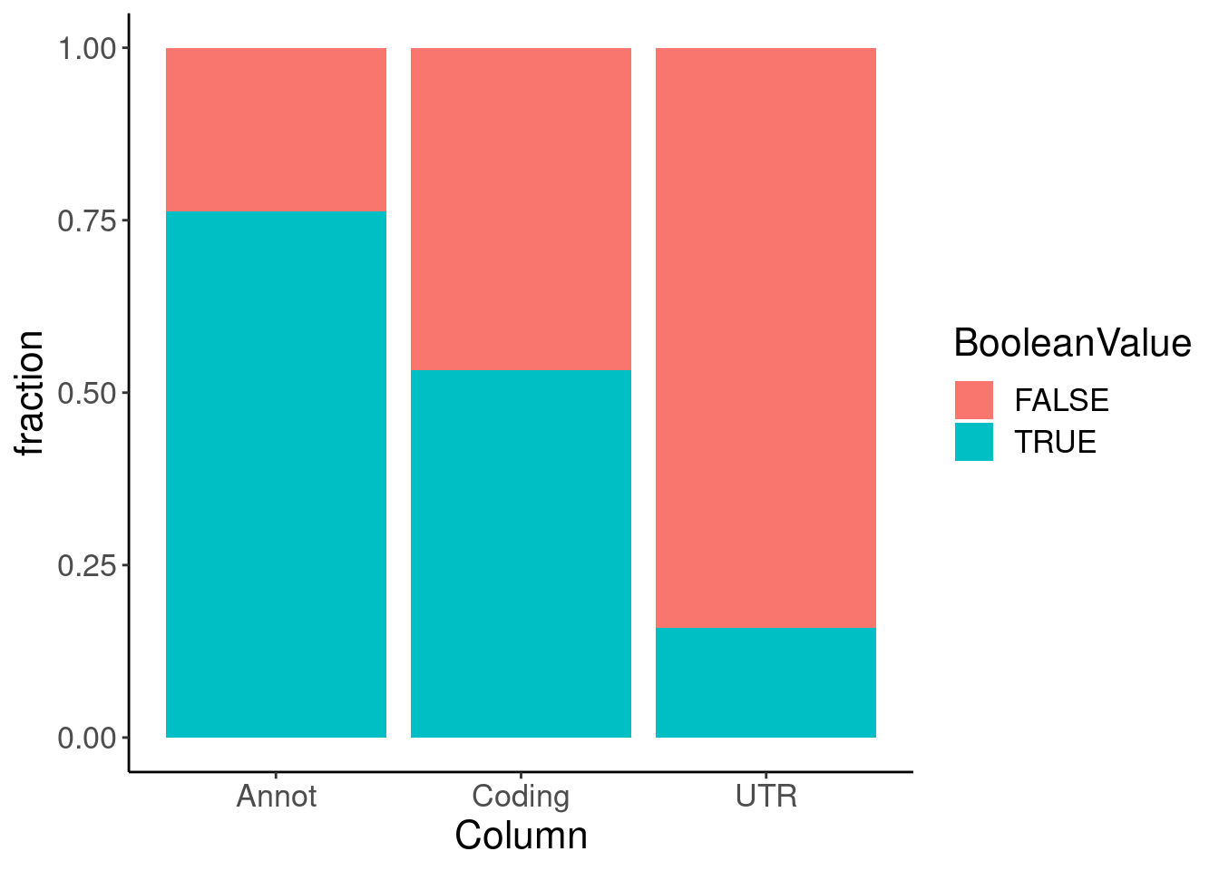

And reminder to self that all UTR junctions (UTR==TRUE) are considered non-coding. Not sure if this is the precise terminology we want in the end… Like UTR junctions are non-coding, but don’t necessarily imply they create a NMD-targeted transcript.

Annotations.filtered %>%
  filter(Coding==F) %>%
  count(UTR)

# A tibble: 2 × 2
  UTR       n
  <lgl> <int>
1 FALSE 91883
2 TRUE  47312

Annotations.filtered %>%
  filter(Coding) %>%
  count(UTR)

# A tibble: 1 × 2
  UTR        n
  <lgl>  <int>
1 FALSE 158604

Annotations.filtered %>%
  filter(UTR) %>%
  count(Coding)

# A tibble: 1 × 2
  Coding     n
  <lgl>  <int>
1 FALSE  47312

Ok, let’s read in our previous intron annotations and compare…

Previous.Annotations <- read_tsv("../data/IntronAnnotationsFromYang.Updated.tsv.gz")

Annotations.filtered.joined <- Annotations.filtered %>%
  inner_join(Previous.Annotations)

Annotations.filtered.joined %>%
  distinct(NewAnnotation)

# A tibble: 31 × 1
   NewAnnotation                     
   <chr>                             
 1 retained_intron.gencode           
 2 protein_coding.gencode            
 3 nonsense_mediated_decay.YN        
 4 processed_transcript.gencode      
 5 nonsense_mediated_decay.pstopcodon
 6 stable.YY                         
 7 nonsense_mediated_decay.far3p     
 8 stable.UTR_junction               
 9 nonsense_mediated_decay.far5p     
10 nonsense_mediated_decay.gencode   
# … with 21 more rows

Annotations.filtered.joined %>%
  distinct(SuperAnnotation)

# A tibble: 6 × 1
  SuperAnnotation                       
  <chr>                                 
1 AnnotatedJunc_UnproductiveCodingGene  
2 AnnotatedJunc_ProductiveCodingGene    
3 UnannotatedJunc_UnproductiveCodingGene
4 UnannotatedJunc_ProductiveCodingGene  
5 AnnotatedJunc_NoncodingGene           
6 UnannotatedJunc_NoncodingJunc         

Annotations.filtered.joined %>%
  count(NewAnnotation, SuperAnnotation,  Annot, Coding, UTR) %>%
  group_by(NewAnnotation) %>%
  mutate(Group_n = sum(n)) %>%
  ungroup() %>%
  mutate(Color = recode(SuperAnnotation, AnnotatedJunc_NoncodingGene="#6a3d9a", UnannotatedJunc_NoncodingJunc="#cab2d6", AnnotatedJunc_UnproductiveCodingGene="#e31a1c", UnannotatedJunc_UnproductiveCodingGene="#fb9a99", AnnotatedJunc_ProductiveCodingGene="#1f78b4", UnannotatedJunc_ProductiveCodingGene="#a6cee3")) %>%
  mutate(groupName = str_glue("n={Group_n}\n{NewAnnotation}")) %>%
  filter(Group_n>50) %>%
  arrange(SuperAnnotation, Group_n) %>%
  pivot_longer(names_to = "Column", values_to = "BooleanValue",  c("Annot", "Coding", "UTR")) %>%
  ggplot() +
    geom_col(aes(x=Column, y=n, fill=BooleanValue), position='fill') +
    geom_rect(data = . %>%
                distinct(groupName, Color,.keep_all=T), alpha=0,
              xmin=-Inf, xmax=Inf, ymin=-Inf, ymax=Inf, size=3, aes(color=Color)) +
   scale_color_identity() +
    labs(y="fraction") +
    facet_wrap(~groupName, scales="free")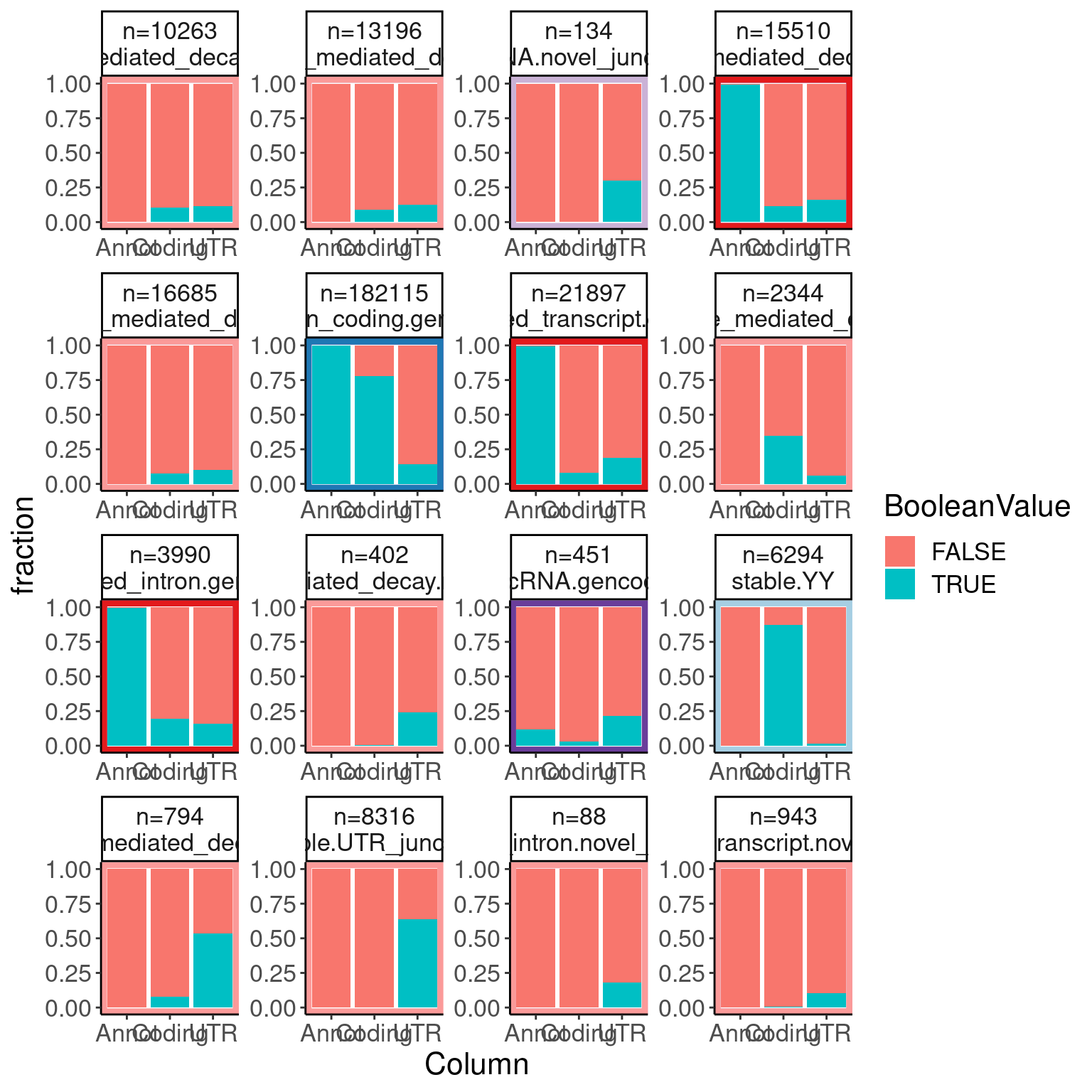

Ok I think those make sense generally. Let’s also look at relative junction usage in naRNA vs steady-state, similar to what we did in a supplement figure with scatter plots of junction RPM.

juncs.long <- fread("../code/SplicingAnalysis/CombinedJuncTables/All.tsv.gz")
dat.KD <- fread("/project2/yangili1/cfbuenabadn/ChromatinSplicingQTLs/code/SplicingAnalysis/CombinedJuncTables/NMD_KD.tsv.gz")


juncs.long.summary <- 
  bind_rows(
    juncs.long,
    dat.KD) %>%
  dplyr::select(chrom, start, stop, strand, Dataset, Count) %>%
  group_by(Dataset, chrom, start, stop) %>%
  summarise(Sum=sum(Count)) %>%
  ungroup()

juncs.long.summary.joined <- juncs.long.summary %>%
  group_by(Dataset) %>%
  mutate(DatasetSum = sum(Sum)) %>%
  ungroup() %>%
  mutate(RPM = Sum/DatasetSum*1E6) %>%
  mutate(stop = stop+1) %>%
  inner_join(Annotations.filtered.joined, by=c("chrom", "start", "stop"="end"))

juncs.long.summary.joined %>%
  distinct(Dataset)

# A tibble: 9 × 1
  Dataset                  
  <chr>                    
1 Expression.Splicing      
2 HeLa.SMG6.KD             
3 HeLa.SMG7.KD             
4 HeLa.UPF1.KD             
5 HeLa.dKD                 
6 HeLa.scr                 
7 MetabolicLabelled.30min  
8 MetabolicLabelled.60min  
9 chRNA.Expression.Splicing

juncs.long.summary.joined %>%
  filter(!UTR) %>%
  filter(Dataset %in% c("Expression.Splicing", "chRNA.Expression.Splicing")) %>%
  dplyr::select(-DatasetSum, -Sum) %>%
  pivot_wider(names_from="Dataset", values_from="RPM") %>%
  mutate(Color = recode(SuperAnnotation, AnnotatedJunc_NoncodingGene="#6a3d9a", UnannotatedJunc_NoncodingJunc="#cab2d6", AnnotatedJunc_UnproductiveCodingGene="#e31a1c", UnannotatedJunc_UnproductiveCodingGene="#fb9a99", AnnotatedJunc_ProductiveCodingGene="#1f78b4", UnannotatedJunc_ProductiveCodingGene="#a6cee3")) %>%
  mutate(SuperAnnotation = factor(SuperAnnotation, levels=c("AnnotatedJunc_ProductiveCodingGene", "UnannotatedJunc_ProductiveCodingGene", "AnnotatedJunc_UnproductiveCodingGene", "UnannotatedJunc_UnproductiveCodingGene", "AnnotatedJunc_NoncodingGene", "UnannotatedJunc_NoncodingJunc"))) %>%
  ggplot(aes(x=Expression.Splicing, y=chRNA.Expression.Splicing)) +
  geom_point(alpha=0.01, color='black') +
  geom_density2d(aes(color=Color)) +
  geom_text(data = . %>%
              replace_na(list(Expression.Splicing=1E-5, chRNA.Expression.Splicing=1E-5)) %>%
              group_by(Coding, SuperAnnotation) %>%
              summarise(med = round(median(chRNA.Expression.Splicing/Expression.Splicing, na.rm=F), 3),
                        n = n()) %>%
              ungroup(),
            aes(label=str_glue("med={med}\nn={n}")),
            x=-Inf, y=Inf, vjust=1, hjust=0.) +
  scale_color_identity() +
  scale_x_continuous(trans="log10", breaks=c(1E-1, 10, 1000), labels=c("0.1", "10", "1000")) +
  scale_y_continuous(trans="log10", breaks=c(1E-1, 10, 1000), labels=c("0.1", "10", "1000")) +
  geom_abline(slope = 1, color='red') +
  facet_grid(Coding~SuperAnnotation) +
  theme_bw() +
  labs(x="Junction RPM, steady-state", y="Junction RPM, chRNA", caption="Filtered out UTR juncs.\nHorizontal facets are 'Coding' value")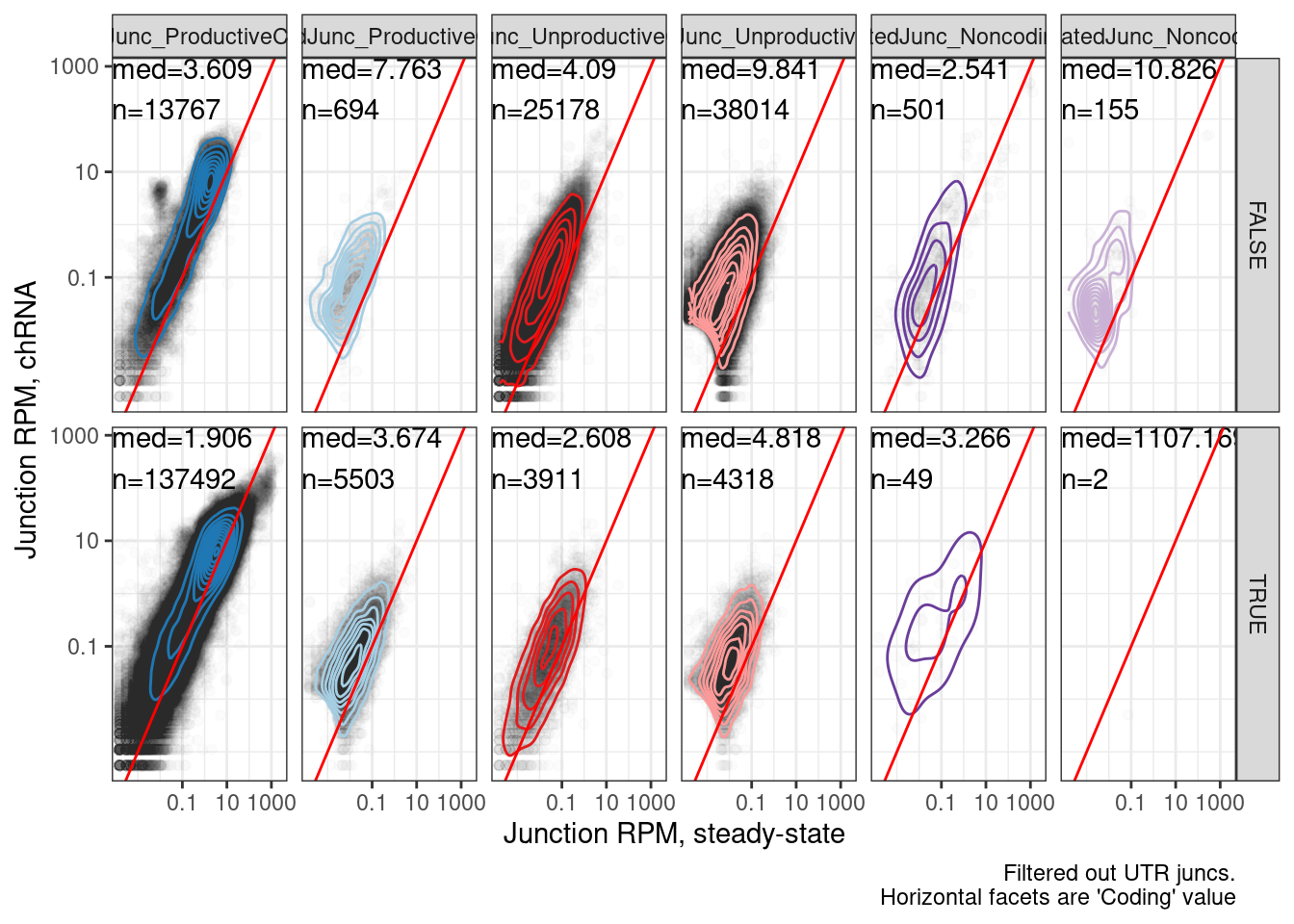

juncs.long.summary.joined %>%
  filter(!UTR) %>%
  filter(Dataset %in% c("HeLa.scr", "HeLa.dKD")) %>%
  dplyr::select(-DatasetSum, -Sum) %>%
  pivot_wider(names_from="Dataset", values_from="RPM") %>%
  mutate(Color = recode(SuperAnnotation, AnnotatedJunc_NoncodingGene="#6a3d9a", UnannotatedJunc_NoncodingJunc="#cab2d6", AnnotatedJunc_UnproductiveCodingGene="#e31a1c", UnannotatedJunc_UnproductiveCodingGene="#fb9a99", AnnotatedJunc_ProductiveCodingGene="#1f78b4", UnannotatedJunc_ProductiveCodingGene="#a6cee3")) %>%
  mutate(SuperAnnotation = factor(SuperAnnotation, levels=c("AnnotatedJunc_ProductiveCodingGene", "UnannotatedJunc_ProductiveCodingGene", "AnnotatedJunc_UnproductiveCodingGene", "UnannotatedJunc_UnproductiveCodingGene", "AnnotatedJunc_NoncodingGene", "UnannotatedJunc_NoncodingJunc"))) %>%
  ggplot(aes(x=HeLa.scr, y=HeLa.dKD)) +
  geom_point(alpha=0.01, color='black') +
  geom_density2d(aes(color=Color)) +
  geom_text(data = . %>%
              replace_na(list(HeLa.scr=1E-5, HeLa.dKD=1E-5)) %>%
              group_by(Coding, SuperAnnotation) %>%
              summarise(med = round(median(HeLa.dKD/HeLa.scr, na.rm=F), 3),
                        n = n()) %>%
              ungroup(),
            aes(label=str_glue("med={med}\nn={n}")),
            x=-Inf, y=Inf, vjust=1, hjust=0.) +
  scale_color_identity() +
  scale_x_continuous(trans="log10", breaks=c(1E-1, 10, 1000), labels=c("0.1", "10", "1000")) +
  scale_y_continuous(trans="log10", breaks=c(1E-1, 10, 1000), labels=c("0.1", "10", "1000")) +
  geom_abline(slope = 1, color='red') +
  facet_grid(Coding~SuperAnnotation) +
  theme_bw() +
  labs(x="Junction RPM, control", y="Junction RPM, dKD", caption="Filtered out UTR juncs.\nHorizontal facets are 'Coding' value")

Response to review

Let’s make similar versions of these plots but now from the long read-determined context of juncs

JuncAnnotationsFromLongReadContext <- read_tsv("../output/20240322_ResponseToReviewerMostCommonJuncContexts.tsv.gz") %>%
  separate(Introns, into=c("chrom", "start", "stop", "strand"), sep="_", convert=T)

juncs.long.summary.joined.LongReadContext <- juncs.long.summary %>%
  group_by(Dataset) %>%
  mutate(DatasetSum = sum(Sum)) %>%
  ungroup() %>%
  mutate(RPM = Sum/DatasetSum*1E6) %>%
  mutate(stop = stop+1) %>%
  inner_join(JuncAnnotationsFromLongReadContext, by=c("chrom", "start", "stop"))

juncs.long.summary.joined.LongReadContext %>%
  distinct(Dataset)

# A tibble: 9 × 1
  Dataset                  
  <chr>                    
1 Expression.Splicing      
2 HeLa.SMG6.KD             
3 HeLa.SMG7.KD             
4 HeLa.UPF1.KD             
5 HeLa.dKD                 
6 HeLa.scr                 
7 MetabolicLabelled.30min  
8 MetabolicLabelled.60min  
9 chRNA.Expression.Splicing

juncs.long.summary.joined.LongReadContext %>%
  filter(Dataset %in% c("Expression.Splicing", "chRNA.Expression.Splicing")) %>%
  dplyr::select(-DatasetSum, -Sum) %>%
  pivot_wider(names_from="Dataset", values_from="RPM") %>%
  mutate(Color = recode(SuperAnnotation, AnnotatedJunc_NoncodingGene="#6a3d9a", UnannotatedJunc_NoncodingJunc="#cab2d6", AnnotatedJunc_UnproductiveCodingGene="#e31a1c", UnannotatedJunc_UnproductiveCodingGene="#fb9a99", AnnotatedJunc_ProductiveCodingGene="#1f78b4", UnannotatedJunc_ProductiveCodingGene="#a6cee3")) %>%
  mutate(SuperAnnotation = factor(SuperAnnotation, levels=c("AnnotatedJunc_ProductiveCodingGene", "UnannotatedJunc_ProductiveCodingGene", "AnnotatedJunc_UnproductiveCodingGene", "UnannotatedJunc_UnproductiveCodingGene", "AnnotatedJunc_NoncodingGene", "UnannotatedJunc_NoncodingJunc"))) %>%
  ggplot(aes(x=Expression.Splicing, y=chRNA.Expression.Splicing)) +
  geom_point(alpha=0.01, color='black') +
  geom_density2d() +
  geom_text(data = . %>%
              replace_na(list(Expression.Splicing=1E-5, chRNA.Expression.Splicing=1E-5)) %>%
              group_by(ModeNMDFinder, SuperAnnotation) %>%
              summarise(med = round(median(chRNA.Expression.Splicing/Expression.Splicing, na.rm=F), 3),
                        n = n()) %>%
              ungroup(),
            aes(label=str_glue("med={med}\nn={n}")),
            x=-Inf, y=Inf, vjust=1, hjust=0.) +
  scale_color_identity() +
  scale_x_continuous(trans="log10", breaks=c(1E-1, 10, 1000), labels=c("0.1", "10", "1000")) +
  scale_y_continuous(trans="log10", breaks=c(1E-1, 10, 1000), labels=c("0.1", "10", "1000")) +
  geom_abline(slope = 1, color='red') +
  facet_grid(ModeNMDFinder~SuperAnnotation) +
  theme_bw() +
  labs(x="Junction RPM, steady-state", y="Junction RPM, chRNA")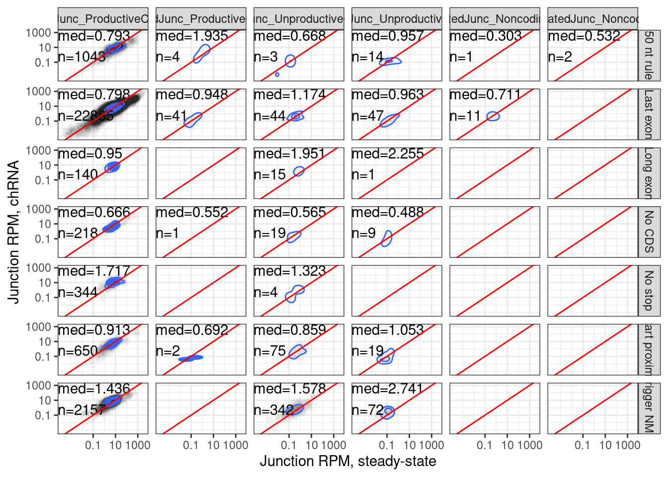

juncs.long.summary.joined.LongReadContext %>%
  filter(Dataset %in% c("HeLa.scr", "HeLa.dKD")) %>%
  dplyr::select(-DatasetSum, -Sum) %>%
  pivot_wider(names_from="Dataset", values_from="RPM") %>%
  mutate(Color = recode(SuperAnnotation, AnnotatedJunc_NoncodingGene="#6a3d9a", UnannotatedJunc_NoncodingJunc="#cab2d6", AnnotatedJunc_UnproductiveCodingGene="#e31a1c", UnannotatedJunc_UnproductiveCodingGene="#fb9a99", AnnotatedJunc_ProductiveCodingGene="#1f78b4", UnannotatedJunc_ProductiveCodingGene="#a6cee3")) %>%
  mutate(SuperAnnotation = factor(SuperAnnotation, levels=c("AnnotatedJunc_ProductiveCodingGene", "UnannotatedJunc_ProductiveCodingGene", "AnnotatedJunc_UnproductiveCodingGene", "UnannotatedJunc_UnproductiveCodingGene", "AnnotatedJunc_NoncodingGene", "UnannotatedJunc_NoncodingJunc"))) %>%
  ggplot(aes(x=HeLa.scr, y=HeLa.dKD)) +
  geom_point(alpha=0.01, color='black') +
  geom_density2d() +
  geom_text(data = . %>%
              replace_na(list(HeLa.scr=1E-5, HeLa.dKD=1E-5)) %>%
              group_by(ModeNMDFinder, SuperAnnotation) %>%
              summarise(med = round(median(HeLa.dKD/HeLa.scr, na.rm=F), 3),
                        n = n()) %>%
              ungroup(),
            aes(label=str_glue("med={med}\nn={n}")),
            x=-Inf, y=Inf, vjust=1, hjust=0.) +
  scale_color_identity() +
  scale_x_continuous(trans="log10", breaks=c(1E-1, 10, 1000), labels=c("0.1", "10", "1000")) +
  scale_y_continuous(trans="log10", breaks=c(1E-1, 10, 1000), labels=c("0.1", "10", "1000")) +
  geom_abline(slope = 1, color='red') +
  facet_grid(ModeNMDFinder~SuperAnnotation) +
  theme_bw() +
  labs(x="Junction RPM, control", y="Junction RPM, dKD")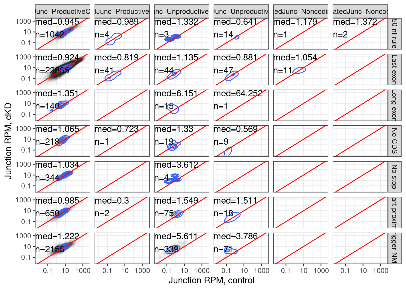

…same thing but now just disregard the old categories

juncs.long.summary.joined.LongReadContext %>%
  filter(Dataset %in% c("Expression.Splicing", "chRNA.Expression.Splicing")) %>%
  dplyr::select(-DatasetSum, -Sum) %>%
  pivot_wider(names_from="Dataset", values_from="RPM") %>%
  ggplot(aes(x=Expression.Splicing, y=chRNA.Expression.Splicing)) +
  geom_point(alpha=0.01, color='black') +
  geom_density2d() +
  geom_text(data = . %>%
              replace_na(list(Expression.Splicing=1E-5, chRNA.Expression.Splicing=1E-5)) %>%
              group_by(ModeNMDFinder) %>%
              summarise(med = round(median(chRNA.Expression.Splicing/Expression.Splicing, na.rm=F), 3),
                        n = n()) %>%
              ungroup(),
            aes(label=str_glue("med={med}\nn={n}")),
            x=-Inf, y=Inf, vjust=1, hjust=0.) +
  scale_color_identity() +
  scale_x_continuous(trans="log10", breaks=c(1E-1, 10, 1000), labels=c("0.1", "10", "1000")) +
  scale_y_continuous(trans="log10", breaks=c(1E-1, 10, 1000), labels=c("0.1", "10", "1000")) +
  geom_abline(slope = 1, color='red') +
  facet_wrap(~ModeNMDFinder) +
  theme_bw() +
  labs(x="Junction RPM, steady-state", y="Junction RPM, chRNA")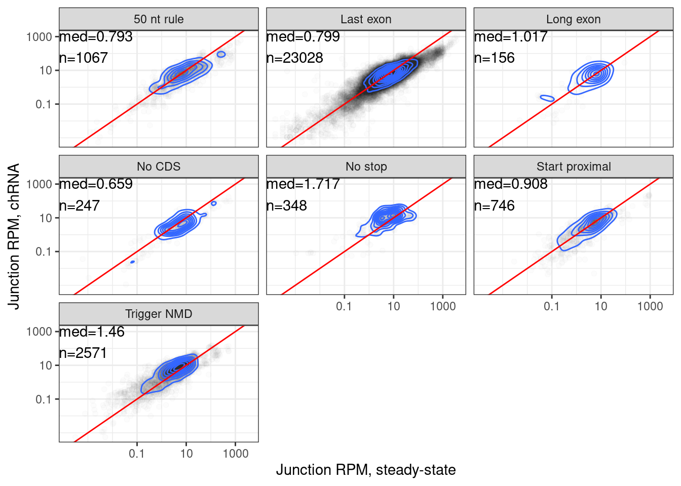

juncs.long.summary.joined.LongReadContext %>%
  filter(Dataset %in% c("HeLa.scr", "HeLa.dKD")) %>%
  dplyr::select(-DatasetSum, -Sum) %>%
  pivot_wider(names_from="Dataset", values_from="RPM") %>%
  ggplot(aes(x=HeLa.scr, y=HeLa.dKD)) +
  geom_point(alpha=0.01, color='black') +
  geom_density2d() +
  geom_text(data = . %>%
              replace_na(list(HeLa.scr=1E-5, HeLa.dKD=1E-5)) %>%
              group_by(ModeNMDFinder) %>%
              summarise(med = round(median(HeLa.dKD/HeLa.scr, na.rm=F), 3),
                        n = n()) %>%
              ungroup(),
            aes(label=str_glue("med={med}\nn={n}")),
            x=-Inf, y=Inf, vjust=1, hjust=0.) +
  scale_color_identity() +
  scale_x_continuous(trans="log10", breaks=c(1E-1, 10, 1000), labels=c("0.1", "10", "1000")) +
  scale_y_continuous(trans="log10", breaks=c(1E-1, 10, 1000), labels=c("0.1", "10", "1000")) +
  geom_abline(slope = 1, color='red') +
  facet_wrap(~ModeNMDFinder) +
  theme_bw() +
  labs(x="Junction RPM, control", y="Junction RPM, dKD")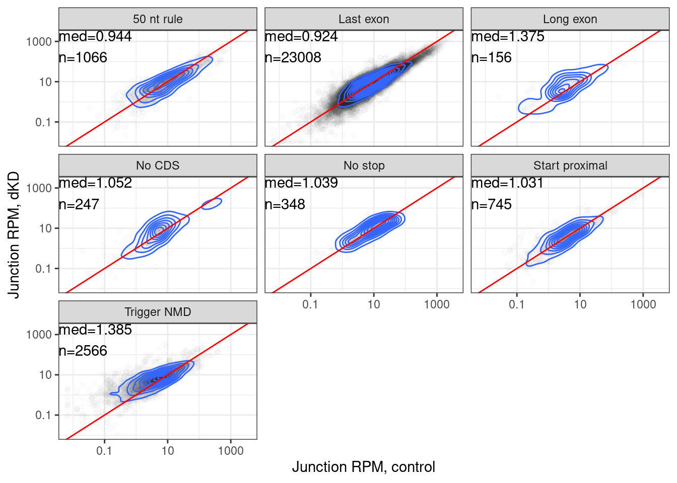

Ok let’s plot these median fold enrichments as a heatmap, since it is totally consistent with the levels of NMD efficiency observed in Lindeboom et al.

NMD.Efficiency.P.dat <- bind_rows(
  juncs.long.summary.joined.LongReadContext %>%
    filter(Dataset %in% c("Expression.Splicing", "chRNA.Expression.Splicing")) %>%
    dplyr::select(-DatasetSum, -Sum) %>%
    pivot_wider(names_from="Dataset", values_from="RPM") %>%
    replace_na(list(Expression.Splicing=1E-5, chRNA.Expression.Splicing=1E-5)) %>%
    group_by(ModeNMDFinder) %>%
    summarise(med = log2(median(chRNA.Expression.Splicing/Expression.Splicing, na.rm=F))) %>%
    ungroup() %>%
    mutate(Comparison = "log2(naRNA/SteadyState)"),
  juncs.long.summary.joined.LongReadContext %>%
  filter(Dataset %in% c("HeLa.scr", "HeLa.dKD")) %>%
    dplyr::select(-DatasetSum, -Sum) %>%
    pivot_wider(names_from="Dataset", values_from="RPM") %>%
    replace_na(list(HeLa.scr=1E-5, HeLa.dKD=1E-5)) %>%
    group_by(ModeNMDFinder) %>%
    summarise(med = log2(median(HeLa.dKD/HeLa.scr, na.rm=F))) %>%
    ungroup() %>%
    mutate(Comparison = "log2(HeLa.dKD/HeLa.scr)")
)

NMD.Efficiency.P.dat %>%
  inner_join(NMD.Efficiency.P.dat %>%
               filter(ModeNMDFinder == "Last exon") %>%
               dplyr::select(LastExonMed = med, Comparison)) %>%
  mutate(MedEffectRelativeToLastExonMed = med - LastExonMed) %>%
  mutate(ModeNMDFinder = factor(ModeNMDFinder, levels=c("Last exon", "50 nt rule", "Start proximal",  "Long exon", "Trigger NMD", "No stop", "No CDS"))) %>%
  mutate(Comparison = recode(Comparison, "log2(HeLa.dKD/HeLa.scr)"=str_wrap("shRNA control\nvs\nshRNA dKD NMD factors", 10), "log2(naRNA/SteadyState)"=str_wrap("steady-state vs naRNA", 20))) %>%
  ggplot(aes(x=Comparison, y=ModeNMDFinder, fill=MedEffectRelativeToLastExonMed)) +
  geom_raster() +
  geom_text(aes(label=round(MedEffectRelativeToLastExonMed, 3))) +
  scale_fill_viridis_c() +
  scale_x_discrete(expand=c(0,0)) +
  scale_y_discrete(expand=c(0,0)) +
  labs(y="Most common full-\ntranscript context", x="Short read datasets for degredation efficiency estimate", fill="Degredation\nefficiency\nestimate")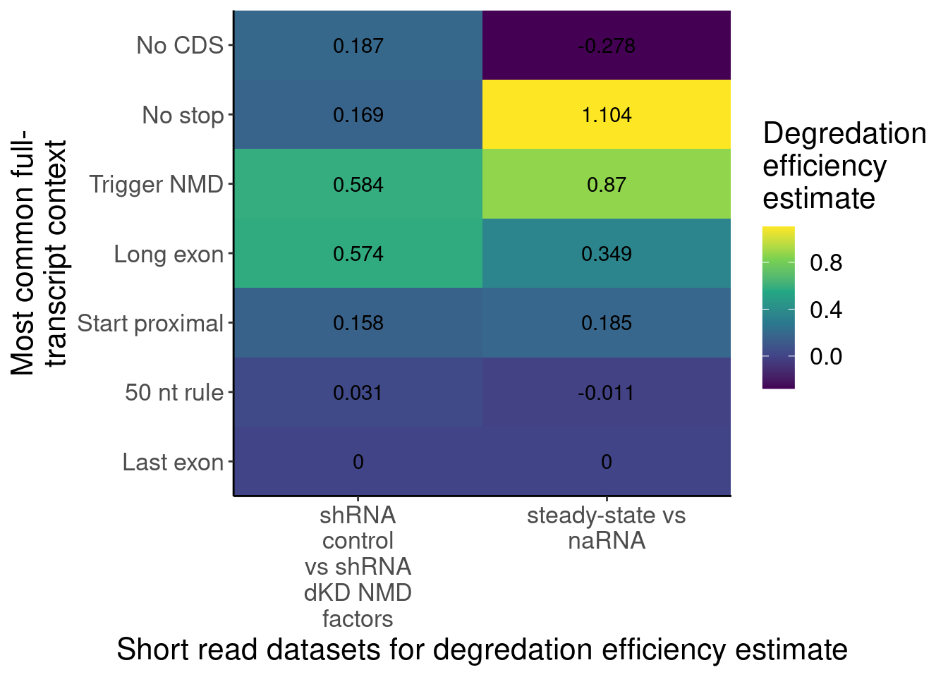

ggsave("/project2/yangili1/carlos_and_ben_shared/rough_figs/OriginalSubplots/202403_ResponseToReviewersDegredationEfficiency.pdf", width=5, height=4)

Head to head plots

Let’s more directly plot the old annotations vs the new annotations to see which method is better (has more enrichment in dKD or chRNA)

juncs.long.summary.joined.toplot <- juncs.long.summary.joined %>%
  filter(!UTR) %>%
  filter(Dataset %in% c("HeLa.scr", "HeLa.dKD")) %>%
  dplyr::select(-DatasetSum, -Sum) %>%
  pivot_wider(names_from="Dataset", values_from="RPM") %>%
  mutate(Color = recode(SuperAnnotation, AnnotatedJunc_NoncodingGene="#6a3d9a", UnannotatedJunc_NoncodingJunc="#cab2d6", AnnotatedJunc_UnproductiveCodingGene="#e31a1c", UnannotatedJunc_UnproductiveCodingGene="#fb9a99", AnnotatedJunc_ProductiveCodingGene="#1f78b4", UnannotatedJunc_ProductiveCodingGene="#a6cee3")) %>%
  mutate(SuperAnnotation = factor(SuperAnnotation, levels=c("AnnotatedJunc_ProductiveCodingGene", "UnannotatedJunc_ProductiveCodingGene", "AnnotatedJunc_UnproductiveCodingGene", "UnannotatedJunc_UnproductiveCodingGene", "AnnotatedJunc_NoncodingGene", "UnannotatedJunc_NoncodingJunc"))) %>%
  filter(!SuperAnnotation %in% c("AnnotatedJunc_NoncodingGene", "UnannotatedJunc_NoncodingJunc"))

bind_rows(
  juncs.long.summary.joined.toplot %>%
    mutate(method="Old"),
  juncs.long.summary.joined.toplot %>%
    mutate(method="New"), 
) %>%
  mutate(ProductiveOrUnproductive = case_when(
    method == "New" ~ Coding,
    method == "Old" & SuperAnnotation %in% c("AnnotatedJunc_ProductiveCodingGene", "UnannotatedJunc_ProductiveCodingGene") ~ TRUE,
    method == "Old" & SuperAnnotation %in% c("AnnotatedJunc_UnproductiveCodingGene", "UnannotatedJunc_UnproductiveCodingGene") ~ FALSE
  )) %>%
  ggplot(aes(x=HeLa.scr, y=HeLa.dKD)) +
  geom_point(alpha=0.01, color='black') +
  geom_density2d(color='red') +
  geom_text(data = . %>%
              replace_na(list(HeLa.scr=1E-5, HeLa.dKD=1E-5)) %>%
              group_by(method, ProductiveOrUnproductive) %>%
              summarise(med = round(median(HeLa.dKD/HeLa.scr, na.rm=F), 3),
                        n = n()) %>%
              ungroup(),
            aes(label=str_glue("med={med}\nn={n}")),
            x=-Inf, y=Inf, vjust=1, hjust=0.) +
  scale_color_identity() +
  scale_x_continuous(trans="log10", breaks=c(1E-1, 10, 1000), labels=c("0.1", "10", "1000")) +
  scale_y_continuous(trans="log10", breaks=c(1E-1, 10, 1000), labels=c("0.1", "10", "1000")) +
  geom_abline(slope = 1, color='red') +
  facet_grid(method~ProductiveOrUnproductive) +
  theme_bw() +
  labs(x="Junction RPM, control", y="Junction RPM, dKD", caption="Filtered out UTR juncs.\nVertical facets are 'Coding' value")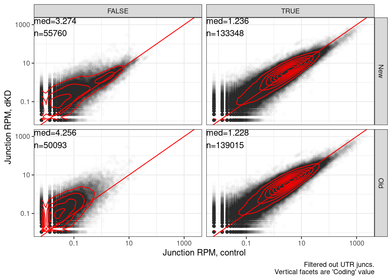

Same plot but steady state vs chRNA…

juncs.long.summary.joined.toplot <- juncs.long.summary.joined %>%
  filter(!UTR) %>%
  filter(Dataset %in% c("Expression.Splicing", "chRNA.Expression.Splicing")) %>%
  dplyr::select(-DatasetSum, -Sum) %>%
  pivot_wider(names_from="Dataset", values_from="RPM") %>%
  mutate(Color = recode(SuperAnnotation, AnnotatedJunc_NoncodingGene="#6a3d9a", UnannotatedJunc_NoncodingJunc="#cab2d6", AnnotatedJunc_UnproductiveCodingGene="#e31a1c", UnannotatedJunc_UnproductiveCodingGene="#fb9a99", AnnotatedJunc_ProductiveCodingGene="#1f78b4", UnannotatedJunc_ProductiveCodingGene="#a6cee3")) %>%
  mutate(SuperAnnotation = factor(SuperAnnotation, levels=c("AnnotatedJunc_ProductiveCodingGene", "UnannotatedJunc_ProductiveCodingGene", "AnnotatedJunc_UnproductiveCodingGene", "UnannotatedJunc_UnproductiveCodingGene", "AnnotatedJunc_NoncodingGene", "UnannotatedJunc_NoncodingJunc"))) %>%
  filter(!SuperAnnotation %in% c("AnnotatedJunc_NoncodingGene", "UnannotatedJunc_NoncodingJunc"))

bind_rows(
  juncs.long.summary.joined.toplot %>%
    mutate(method="Old"),
  juncs.long.summary.joined.toplot %>%
    mutate(method="New"), 
) %>%
  mutate(ProductiveOrUnproductive = case_when(
    method == "New" ~ Coding,
    method == "Old" & SuperAnnotation %in% c("AnnotatedJunc_ProductiveCodingGene", "UnannotatedJunc_ProductiveCodingGene") ~ TRUE,
    method == "Old" & SuperAnnotation %in% c("AnnotatedJunc_UnproductiveCodingGene", "UnannotatedJunc_UnproductiveCodingGene") ~ FALSE
  )) %>%
  ggplot(aes(x=Expression.Splicing, y=chRNA.Expression.Splicing)) +
  geom_point(alpha=0.01, color='black') +
  geom_density2d(color='red') +
  geom_text(data = . %>%
              replace_na(list(Expression.Splicing=1E-5, chRNA.Expression.Splicing=1E-5)) %>%
              group_by(method, ProductiveOrUnproductive) %>%
              summarise(med = round(median(chRNA.Expression.Splicing/Expression.Splicing, na.rm=F), 3),
                        n = n()) %>%
              ungroup(),
            aes(label=str_glue("med={med}\nn={n}")),
            x=-Inf, y=Inf, vjust=1, hjust=0.) +
  scale_color_identity() +
  scale_x_continuous(trans="log10", breaks=c(1E-1, 10, 1000), labels=c("0.1", "10", "1000")) +
  scale_y_continuous(trans="log10", breaks=c(1E-1, 10, 1000), labels=c("0.1", "10", "1000")) +
  geom_abline(slope = 1, color='red') +
  facet_grid(method~ProductiveOrUnproductive) +
  theme_bw() +
  labs(x="Junction RPM, steady-state", y="Junction RPM, chRNA", caption="Filtered out UTR juncs.\nVertical facets are 'Coding' value")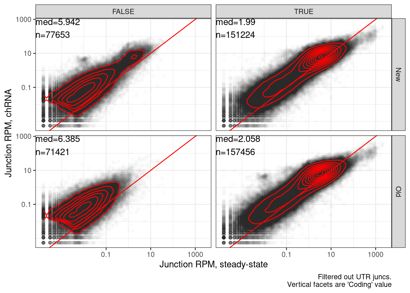

Head to head, with more inclusive for new coding method

Yang suggested tweaking the New classification to also include all annotated productive juncs and productive. So an or statement… here is pseudocode: IsProductiveInNewMethod = (Coding==True OR AnnotatedProductive==TRUE). Now let’s remake those head to head plots…

juncs.long.summary.joined.toplot <- juncs.long.summary.joined %>%
  filter(!UTR) %>%
  filter(Dataset %in% c("HeLa.scr", "HeLa.dKD")) %>%
  dplyr::select(-DatasetSum, -Sum) %>%
  pivot_wider(names_from="Dataset", values_from="RPM") %>%
  mutate(Color = recode(SuperAnnotation, AnnotatedJunc_NoncodingGene="#6a3d9a", UnannotatedJunc_NoncodingJunc="#cab2d6", AnnotatedJunc_UnproductiveCodingGene="#e31a1c", UnannotatedJunc_UnproductiveCodingGene="#fb9a99", AnnotatedJunc_ProductiveCodingGene="#1f78b4", UnannotatedJunc_ProductiveCodingGene="#a6cee3")) %>%
  mutate(SuperAnnotation = factor(SuperAnnotation, levels=c("AnnotatedJunc_ProductiveCodingGene", "UnannotatedJunc_ProductiveCodingGene", "AnnotatedJunc_UnproductiveCodingGene", "UnannotatedJunc_UnproductiveCodingGene", "AnnotatedJunc_NoncodingGene", "UnannotatedJunc_NoncodingJunc"))) %>%
  filter(!SuperAnnotation %in% c("AnnotatedJunc_NoncodingGene", "UnannotatedJunc_NoncodingJunc"))

bind_rows(
  juncs.long.summary.joined.toplot %>%
    mutate(method="Old"),
  juncs.long.summary.joined.toplot %>%
    mutate(method="New"), 
) %>%
  mutate(ProductiveOrUnproductive = case_when(
    method == "New" & (Coding | SuperAnnotation=="AnnotatedJunc_ProductiveCodingGene") ~ TRUE,
    method == "New" & !(Coding | SuperAnnotation=="AnnotatedJunc_ProductiveCodingGene") ~ FALSE,
    method == "Old" & SuperAnnotation %in% c("AnnotatedJunc_ProductiveCodingGene", "UnannotatedJunc_ProductiveCodingGene") ~ TRUE,
    method == "Old" & SuperAnnotation %in% c("AnnotatedJunc_UnproductiveCodingGene", "UnannotatedJunc_UnproductiveCodingGene") ~ FALSE
  )) %>%
  ggplot(aes(x=HeLa.scr, y=HeLa.dKD)) +
  geom_point(alpha=0.01, color='black') +
  geom_density2d(color='red') +
  geom_text(data = . %>%
              replace_na(list(HeLa.scr=1E-5, HeLa.dKD=1E-5)) %>%
              group_by(method, ProductiveOrUnproductive) %>%
              summarise(med = round(median(HeLa.dKD/HeLa.scr, na.rm=F), 3),
                        n = n()) %>%
              ungroup(),
            aes(label=str_glue("med={med}\nn={n}")),
            x=-Inf, y=Inf, vjust=1, hjust=0.) +
  scale_color_identity() +
  scale_x_continuous(trans="log10", breaks=c(1E-1, 10, 1000), labels=c("0.1", "10", "1000")) +
  scale_y_continuous(trans="log10", breaks=c(1E-1, 10, 1000), labels=c("0.1", "10", "1000")) +
  geom_abline(slope = 1, color='red') +
  facet_grid(method~ProductiveOrUnproductive) +
  theme_bw() +
  labs(x="Junction RPM, control", y="Junction RPM, dKD", caption="Filtered out UTR juncs.\nVertical facets are 'Coding' value")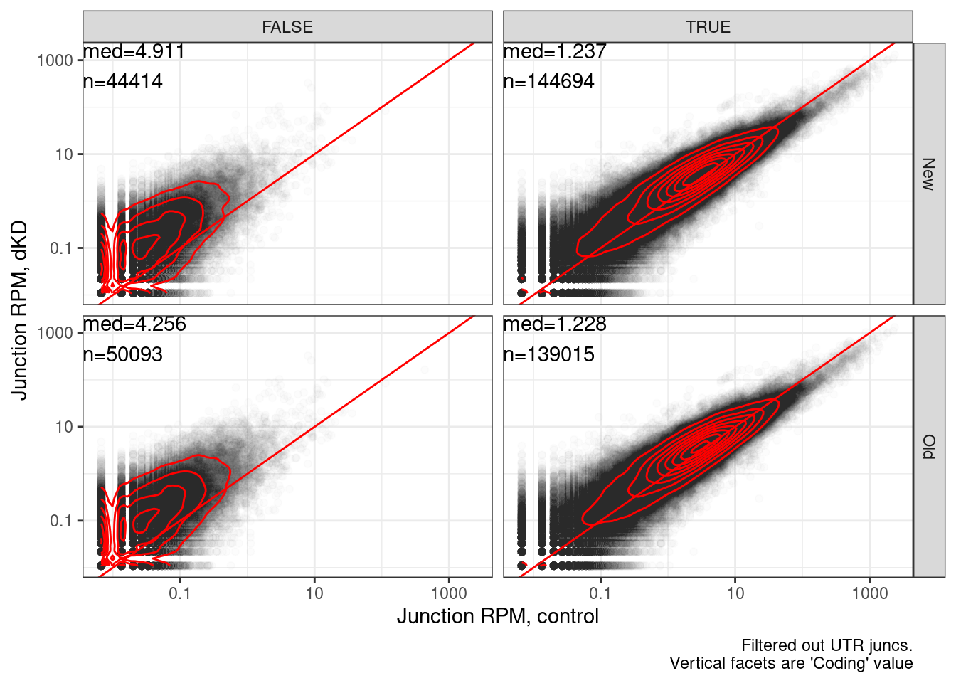

Same plot but steady state vs chRNA…

juncs.long.summary.joined.toplot <- juncs.long.summary.joined %>%
  filter(!UTR) %>%
  filter(Dataset %in% c("Expression.Splicing", "chRNA.Expression.Splicing")) %>%
  dplyr::select(-DatasetSum, -Sum) %>%
  pivot_wider(names_from="Dataset", values_from="RPM") %>%
  mutate(Color = recode(SuperAnnotation, AnnotatedJunc_NoncodingGene="#6a3d9a", UnannotatedJunc_NoncodingJunc="#cab2d6", AnnotatedJunc_UnproductiveCodingGene="#e31a1c", UnannotatedJunc_UnproductiveCodingGene="#fb9a99", AnnotatedJunc_ProductiveCodingGene="#1f78b4", UnannotatedJunc_ProductiveCodingGene="#a6cee3")) %>%
  mutate(SuperAnnotation = factor(SuperAnnotation, levels=c("AnnotatedJunc_ProductiveCodingGene", "UnannotatedJunc_ProductiveCodingGene", "AnnotatedJunc_UnproductiveCodingGene", "UnannotatedJunc_UnproductiveCodingGene", "AnnotatedJunc_NoncodingGene", "UnannotatedJunc_NoncodingJunc"))) %>%
  filter(!SuperAnnotation %in% c("AnnotatedJunc_NoncodingGene", "UnannotatedJunc_NoncodingJunc"))

bind_rows(
  juncs.long.summary.joined.toplot %>%
    mutate(method="Old"),
  juncs.long.summary.joined.toplot %>%
    mutate(method="New"), 
) %>%
  mutate(ProductiveOrUnproductive = case_when(
    method == "New" & (Coding | SuperAnnotation=="AnnotatedJunc_ProductiveCodingGene") ~ TRUE,
    method == "New" & !(Coding | SuperAnnotation=="AnnotatedJunc_ProductiveCodingGene") ~ FALSE,
    method == "Old" & SuperAnnotation %in% c("AnnotatedJunc_ProductiveCodingGene", "UnannotatedJunc_ProductiveCodingGene") ~ TRUE,
    method == "Old" & SuperAnnotation %in% c("AnnotatedJunc_UnproductiveCodingGene", "UnannotatedJunc_UnproductiveCodingGene") ~ FALSE
  )) %>%
  ggplot(aes(x=Expression.Splicing, y=chRNA.Expression.Splicing)) +
  geom_point(alpha=0.01, color='black') +
  geom_density2d(color='red') +
  geom_text(data = . %>%
              replace_na(list(Expression.Splicing=1E-5, chRNA.Expression.Splicing=1E-5)) %>%
              group_by(method, ProductiveOrUnproductive) %>%
              summarise(med = round(median(chRNA.Expression.Splicing/Expression.Splicing, na.rm=F), 3),
                        n = n()) %>%
              ungroup(),
            aes(label=str_glue("med={med}\nn={n}")),
            x=-Inf, y=Inf, vjust=1, hjust=0.) +
  scale_color_identity() +
  scale_x_continuous(trans="log10", breaks=c(1E-1, 10, 1000), labels=c("0.1", "10", "1000")) +
  scale_y_continuous(trans="log10", breaks=c(1E-1, 10, 1000), labels=c("0.1", "10", "1000")) +
  geom_abline(slope = 1, color='red') +
  facet_grid(method~ProductiveOrUnproductive) +
  theme_bw() +
  labs(x="Junction RPM, steady-state", y="Junction RPM, naRNA")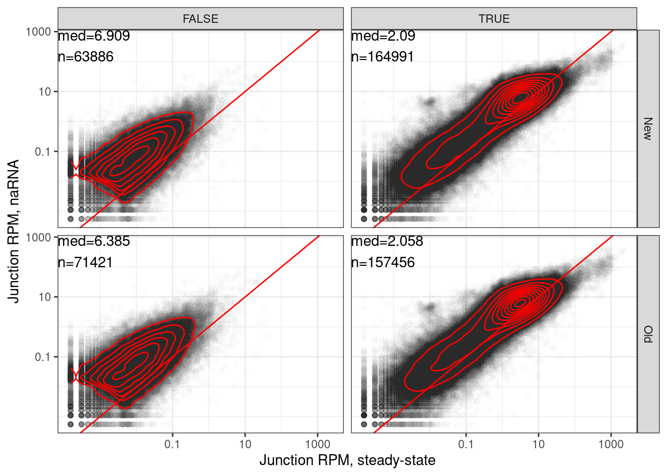

…same plot but just new method

dat.to.Plot <- juncs.long.summary.joined.toplot %>%
  mutate(ProductiveOrUnproductive = case_when(
    (Coding | SuperAnnotation=="AnnotatedJunc_ProductiveCodingGene") ~ "Productive\nSplice juncs",
    !(Coding | SuperAnnotation=="AnnotatedJunc_ProductiveCodingGene") ~ "Unproductive\nSplice juncs",
  ))

ggplot(dat.to.Plot, aes(x=Expression.Splicing, y=chRNA.Expression.Splicing)) +
  geom_point(alpha=0.01, color='black') +
  geom_density2d(color='red') +
  geom_abline(slope = 1, color='red') +
  geom_text(data = . %>%
              replace_na(list(Expression.Splicing=1E-5, chRNA.Expression.Splicing=1E-5)) %>%
              group_by(ProductiveOrUnproductive) %>%
              summarise(med = round(median(chRNA.Expression.Splicing/Expression.Splicing, na.rm=F), 3),
                        n = n()) %>%
              ungroup(),
            aes(label=str_glue("median FC={med}\nn={n}")),
            x=-Inf, y=Inf, vjust=1.1, hjust=0.) +
  scale_color_identity() +
  scale_x_continuous(trans="log10", breaks=c(1E-1, 10, 1000), labels=c("0.1", "10", "1000")) +
  scale_y_continuous(trans="log10", breaks=c(1E-1, 10, 1000), labels=c("0.1", "10", "1000")) +
  facet_wrap(~ProductiveOrUnproductive) +
  theme_bw() +
  coord_fixed() +
  labs(x="Junction RPM, steady-state", y="Junction RPM, naRNA")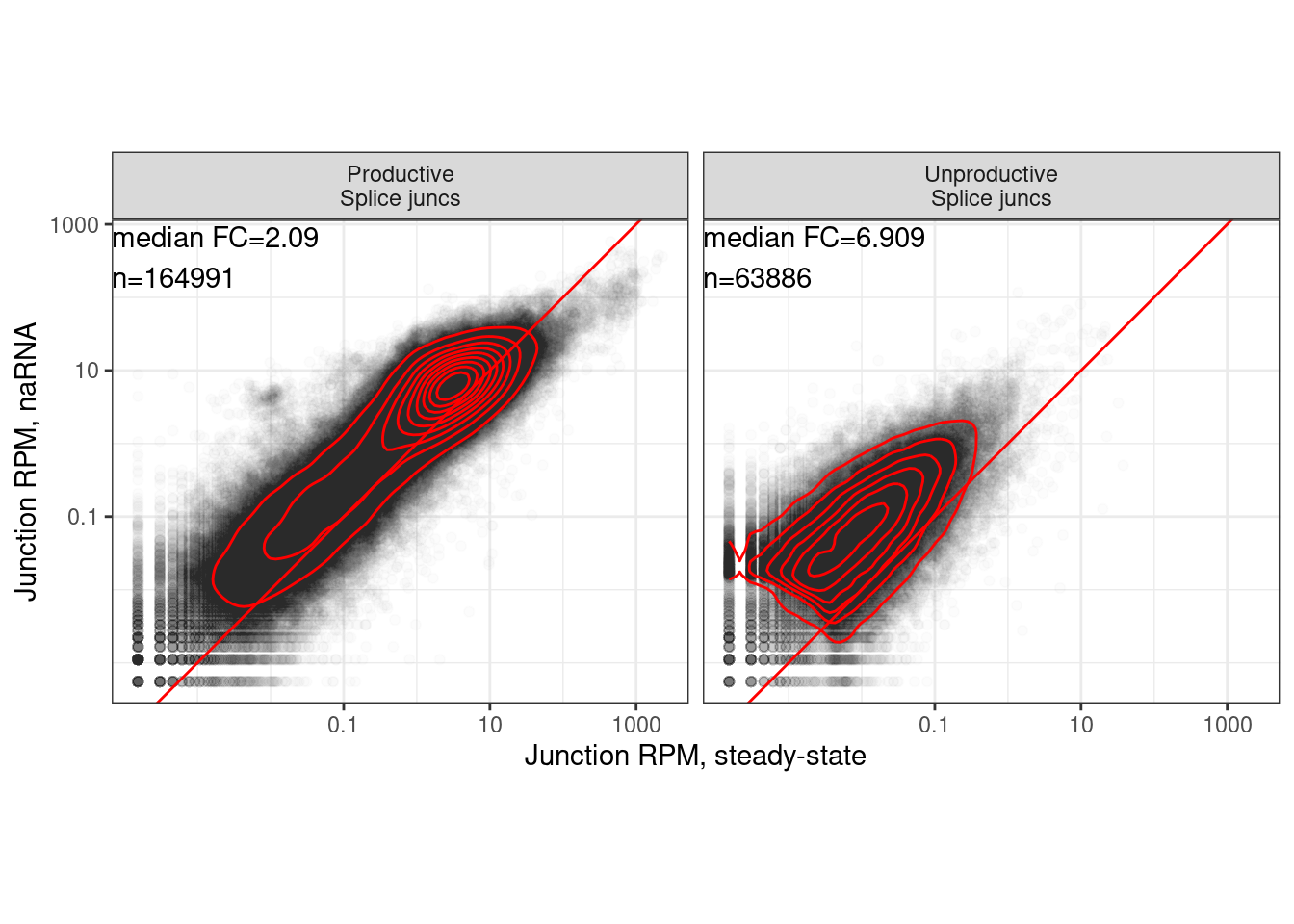

ggsave("../code/scratch/PlotsForYangGrant.JunctionScatter.Points.pdf", height=3, width=7)

ggplot(dat.to.Plot, aes(x=Expression.Splicing, y=chRNA.Expression.Splicing)) +
  # geom_point(alpha=0.01, color='black') +
  # geom_density2d(color='red') +
  geom_hex(bins=70) +
  geom_abline(slope = 1, color='red') +
  geom_text(data = . %>%
              replace_na(list(Expression.Splicing=1E-5, chRNA.Expression.Splicing=1E-5)) %>%
              group_by(ProductiveOrUnproductive) %>%
              summarise(med = round(median(chRNA.Expression.Splicing/Expression.Splicing, na.rm=F), 3),
                        n = n()) %>%
              ungroup(),
            aes(label=str_glue(" median FC={med}\n n={n}")),
            x=-Inf, y=Inf, vjust=1.1, hjust=0.) +
  scale_color_identity() +
  scale_fill_viridis_c(trans='log10', option = 'B') + 
  scale_x_continuous(trans="log10", breaks=c(1E-1, 10, 1000), labels=c("0.1", "10", "1000")) +
  scale_y_continuous(trans="log10", breaks=c(1E-1, 10, 1000), labels=c("0.1", "10", "1000")) +
  facet_wrap(~ProductiveOrUnproductive) +
  theme_bw() +
  coord_fixed() +
  labs(x="Junction RPM, steady-state", y="Junction RPM, naRNA")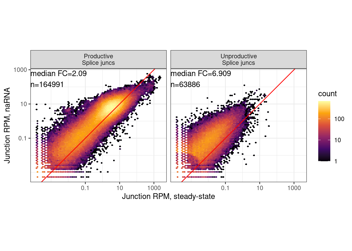

ggsave("../code/scratch/PlotsForYangGrant.JunctionScatter.Hexbin.pdf", height=2, width=4.25)

Plots for Yang’s grant.

juncs.long.summary.joined.toplot <- juncs.long.summary.joined %>%
  filter(!UTR) %>%
  filter(Dataset %in% c("HeLa.scr", "HeLa.dKD")) %>%
  dplyr::select(-DatasetSum, -Sum) %>%
  pivot_wider(names_from="Dataset", values_from="RPM") %>%
  mutate(Color = recode(SuperAnnotation, AnnotatedJunc_NoncodingGene="#6a3d9a", UnannotatedJunc_NoncodingJunc="#cab2d6", AnnotatedJunc_UnproductiveCodingGene="#e31a1c", UnannotatedJunc_UnproductiveCodingGene="#fb9a99", AnnotatedJunc_ProductiveCodingGene="#1f78b4", UnannotatedJunc_ProductiveCodingGene="#a6cee3")) %>%
  mutate(SuperAnnotation = factor(SuperAnnotation, levels=c("AnnotatedJunc_ProductiveCodingGene", "UnannotatedJunc_ProductiveCodingGene", "AnnotatedJunc_UnproductiveCodingGene", "UnannotatedJunc_UnproductiveCodingGene", "AnnotatedJunc_NoncodingGene", "UnannotatedJunc_NoncodingJunc"))) %>%
  filter(!SuperAnnotation %in% c("AnnotatedJunc_NoncodingGene", "UnannotatedJunc_NoncodingJunc"))

bind_rows(
  juncs.long.summary.joined.toplot %>%
    mutate(method="Old"),
  juncs.long.summary.joined.toplot %>%
    mutate(method="New"), 
) %>%
  mutate(ProductiveOrUnproductive = case_when(
    method == "New" & (Coding | SuperAnnotation=="AnnotatedJunc_ProductiveCodingGene") ~ TRUE,
    method == "New" & !(Coding | SuperAnnotation=="AnnotatedJunc_ProductiveCodingGene") ~ FALSE,
    method == "Old" & SuperAnnotation %in% c("AnnotatedJunc_ProductiveCodingGene", "UnannotatedJunc_ProductiveCodingGene") ~ TRUE,
    method == "Old" & SuperAnnotation %in% c("AnnotatedJunc_UnproductiveCodingGene", "UnannotatedJunc_UnproductiveCodingGene") ~ FALSE
  )) %>%
  mutate(ProductiveOrUnproductive = if_else(ProductiveOrUnproductive, "Productive", "Unproductive")) %>%
  ggplot(aes(x=HeLa.scr, y=HeLa.dKD)) +
  # geom_scattermore(alpha=0.01, color='black') +
  # geom_hex() +
  # scale_fill_viridis_c()
  geom_point(alpha=0.01, color='black') +
  geom_density2d(color='red') +
  geom_text(data = . %>%
              replace_na(list(HeLa.scr=1E-5, HeLa.dKD=1E-5)) %>%
              group_by(method, ProductiveOrUnproductive) %>%
              summarise(med = round(median(HeLa.dKD/HeLa.scr, na.rm=F), 3),
                        n = n()) %>%
              ungroup(),
            aes(label=str_glue("Med={med}\nn={n}")),
            x=-Inf, y=Inf, vjust=1, hjust=0.) +
  scale_color_identity() +
  scale_x_continuous(trans="log10", breaks=c(1E-1, 10, 1000), labels=c("0.1", "10", "1000")) +
  scale_y_continuous(trans="log10", breaks=c(1E-1, 10, 1000), labels=c("0.1", "10", "1000")) +
  geom_abline(slope = 1, color='red') +
  facet_grid(method~ProductiveOrUnproductive) +
  theme_classic() +
  labs(x="Junction RPM, control", y="Junction RPM, dKD", caption="Filtered out UTR juncs.\nVertical facets are 'Coding' value")
ggsave("/project2/yangili1/bjf79/scratch/EvaluateJuncClassification.shRNAKD.pdf", height=6, width=3)

bind_rows(
  juncs.long.summary.joined.toplot %>%
    mutate(method="Old"),
  juncs.long.summary.joined.toplot %>%
    mutate(method="New"), 
) %>%
  mutate(ProductiveOrUnproductive = case_when(
    method == "New" & (Coding | SuperAnnotation=="AnnotatedJunc_ProductiveCodingGene") ~ TRUE,
    method == "New" & !(Coding | SuperAnnotation=="AnnotatedJunc_ProductiveCodingGene") ~ FALSE,
    method == "Old" & SuperAnnotation %in% c("AnnotatedJunc_ProductiveCodingGene", "UnannotatedJunc_ProductiveCodingGene") ~ TRUE,
    method == "Old" & SuperAnnotation %in% c("AnnotatedJunc_UnproductiveCodingGene", "UnannotatedJunc_UnproductiveCodingGene") ~ FALSE
  )) %>%
  mutate(ProductiveOrUnproductive = if_else(ProductiveOrUnproductive, "Productive", "Unproductive")) %>%
  filter(method == "New") %>%
  ggplot(aes(x=HeLa.scr, y=HeLa.dKD)) +
  geom_point(alpha=0.01, color='black') +
  geom_density2d(color='red') +
  geom_text(data = . %>%
              replace_na(list(HeLa.scr=1E-5, HeLa.dKD=1E-5)) %>%
              group_by(ProductiveOrUnproductive) %>%
              summarise(med = round(median(HeLa.dKD/HeLa.scr, na.rm=F), 3),
                        n = n()) %>%
              ungroup(),
            aes(label=str_glue("Med={med}\nn={n}")),
            x=-Inf, y=Inf, vjust=1, hjust=0.) +
  scale_color_identity() +
  scale_x_continuous(trans="log10", breaks=c(1E-1, 10, 1000), labels=c("0.1", "10", "1000")) +
  scale_y_continuous(trans="log10", breaks=c(1E-1, 10, 1000), labels=c("0.1", "10", "1000")) +
  geom_abline(slope = 1, color='red') +
  facet_wrap(~ProductiveOrUnproductive) +
  theme_classic() +
  labs(x="Junction RPM, control", y="Junction RPM, dKD", caption="Filtered out UTR juncs.\nVertical facets are 'Coding' value")
# ggsave("/project2/yangili1/bjf79/scratch/EvaluateJuncClassification.shRNAKD.NoOld.pdf", height=3, width=3)





juncs.long.summary.joined.toplot <- juncs.long.summary.joined %>%
  filter(!UTR) %>%
  filter(Dataset %in% c("Expression.Splicing", "chRNA.Expression.Splicing")) %>%
  dplyr::select(-DatasetSum, -Sum) %>%
  pivot_wider(names_from="Dataset", values_from="RPM") %>%
  mutate(Color = recode(SuperAnnotation, AnnotatedJunc_NoncodingGene="#6a3d9a", UnannotatedJunc_NoncodingJunc="#cab2d6", AnnotatedJunc_UnproductiveCodingGene="#e31a1c", UnannotatedJunc_UnproductiveCodingGene="#fb9a99", AnnotatedJunc_ProductiveCodingGene="#1f78b4", UnannotatedJunc_ProductiveCodingGene="#a6cee3")) %>%
  mutate(SuperAnnotation = factor(SuperAnnotation, levels=c("AnnotatedJunc_ProductiveCodingGene", "UnannotatedJunc_ProductiveCodingGene", "AnnotatedJunc_UnproductiveCodingGene", "UnannotatedJunc_UnproductiveCodingGene", "AnnotatedJunc_NoncodingGene", "UnannotatedJunc_NoncodingJunc"))) %>%
  filter(!SuperAnnotation %in% c("AnnotatedJunc_NoncodingGene", "UnannotatedJunc_NoncodingJunc"))

bind_rows(
  juncs.long.summary.joined.toplot %>%
    mutate(method="Old"),
  juncs.long.summary.joined.toplot %>%
    mutate(method="New"), 
) %>%
  mutate(ProductiveOrUnproductive = case_when(
    method == "New" & (Coding | SuperAnnotation=="AnnotatedJunc_ProductiveCodingGene") ~ TRUE,
    method == "New" & !(Coding | SuperAnnotation=="AnnotatedJunc_ProductiveCodingGene") ~ FALSE,
    method == "Old" & SuperAnnotation %in% c("AnnotatedJunc_ProductiveCodingGene", "UnannotatedJunc_ProductiveCodingGene") ~ TRUE,
    method == "Old" & SuperAnnotation %in% c("AnnotatedJunc_UnproductiveCodingGene", "UnannotatedJunc_UnproductiveCodingGene") ~ FALSE
  )) %>%
  mutate(ProductiveOrUnproductive = if_else(ProductiveOrUnproductive, "Productive", "Unproductive")) %>%
  ggplot(aes(x=Expression.Splicing, y=chRNA.Expression.Splicing)) +
  geom_point(alpha=0.01, color='black') +
  geom_density2d(color='red') +
  geom_text(data = . %>%
              replace_na(list(Expression.Splicing=1E-5, chRNA.Expression.Splicing=1E-5)) %>%
              group_by(method, ProductiveOrUnproductive) %>%
              summarise(med = round(median(chRNA.Expression.Splicing/Expression.Splicing, na.rm=F), 3),
                        n = n()) %>%
              ungroup(),
            aes(label=str_glue("Med={med}\nn={n}")),
            x=-Inf, y=Inf, vjust=1, hjust=0.) +
  scale_color_identity() +
  scale_x_continuous(trans="log10", breaks=c(1E-1, 10, 1000), labels=c("0.1", "10", "1000")) +
  scale_y_continuous(trans="log10", breaks=c(1E-1, 10, 1000), labels=c("0.1", "10", "1000")) +
  geom_abline(slope = 1, color='red') +
  facet_grid(method~ProductiveOrUnproductive) +
  theme_classic() +
  labs(x="Junction RPM, steady-state", y="Junction RPM, naRNA", caption="Filtered out UTR juncs.\nVertical facets are 'Coding' value")
# ggsave("/project2/yangili1/bjf79/scratch/EvaluateJuncClassification.naRNA.pdf", height=6, width=3)

bind_rows(
  juncs.long.summary.joined.toplot %>%
    mutate(method="Old"),
  juncs.long.summary.joined.toplot %>%
    mutate(method="New"), 
) %>%
  mutate(ProductiveOrUnproductive = case_when(
    method == "New" & (Coding | SuperAnnotation=="AnnotatedJunc_ProductiveCodingGene") ~ TRUE,
    method == "New" & !(Coding | SuperAnnotation=="AnnotatedJunc_ProductiveCodingGene") ~ FALSE,
    method == "Old" & SuperAnnotation %in% c("AnnotatedJunc_ProductiveCodingGene", "UnannotatedJunc_ProductiveCodingGene") ~ TRUE,
    method == "Old" & SuperAnnotation %in% c("AnnotatedJunc_UnproductiveCodingGene", "UnannotatedJunc_UnproductiveCodingGene") ~ FALSE
  )) %>%
  mutate(ProductiveOrUnproductive = if_else(ProductiveOrUnproductive, "Productive", "Unproductive")) %>%
  filter(method == "New") %>%
  ggplot(aes(x=Expression.Splicing, y=chRNA.Expression.Splicing)) +
  geom_point(alpha=0.01, color='black') +
  geom_density2d(color='red') +
  geom_text(data = . %>%
              replace_na(list(Expression.Splicing=1E-5, chRNA.Expression.Splicing=1E-5)) %>%
              group_by(ProductiveOrUnproductive) %>%
              summarise(med = round(median(chRNA.Expression.Splicing/Expression.Splicing, na.rm=F), 3),
                        n = n()) %>%
              ungroup(),
            aes(label=str_glue("Med={med}\nn={n}")),
            x=-Inf, y=Inf, vjust=1, hjust=0.) +
  scale_color_identity() +
  scale_x_continuous(trans="log10", breaks=c(1E-1, 10, 1000), labels=c("0.1", "10", "1000")) +
  scale_y_continuous(trans="log10", breaks=c(1E-1, 10, 1000), labels=c("0.1", "10", "1000")) +
  geom_abline(slope = 1, color='red') +
  facet_wrap(~ProductiveOrUnproductive) +
  theme_classic() +
  labs(x="Junction RPM, steady-state", y="Junction RPM, naRNA", caption="Filtered out UTR juncs.\nVertical facets are 'Coding' value")
# ggsave("/project2/yangili1/bjf79/scratch/EvaluateJuncClassification.naRNA.NoOld.pdf", height=3, width=3)

Test updated script

Yang updated his script to reflect this new change… I reran the script and now let’s verify the new annotations.

NewScript.Annotations <- read_tsv("/project/yangili1/bjf79/2024_NMD_Junction_Classifier/Leaf2_updated_junction_classifications.txt") %>%
  separate(Intron_coord, into=c("chrom", "start", "end"), sep="[:-]", convert=T, remove = F) %>%
  add_count(Intron_coord, name="NumberOfEntriesWithSameCoords")

juncs.long.summary.joined.toplot %>%
  inner_join(
    NewScript.Annotations %>%
      dplyr::select(Intron_coord, CodingUpdated = Coding)
  ) %>%
  mutate(ProductiveOrUnproductiveMyTest = case_when(
    Coding | SuperAnnotation=="AnnotatedJunc_ProductiveCodingGene" ~ TRUE,
    TRUE ~ FALSE)) %>%
  count(CodingUpdated, ProductiveOrUnproductiveMyTest)

# A tibble: 3 × 3
  CodingUpdated ProductiveOrUnproductiveMyTest      n
  <lgl>         <lgl>                           <int>
1 FALSE         FALSE                           63886
2 FALSE         TRUE                               11
3 TRUE          TRUE                           164980

The script is correctly updated, such that the Coding column in the new srcipt output is true if it can create a transcript that reaches a stop codon, OR if it is already in an annotated functional transcript.

Unrelated code

…To make new metadata file for different project with new sequencing data.

Metadata <- read_tsv("/project2/yangili1/bjf79/sm_splicingmodulators/code/config/samples.tsv")

NewFastq <- read_tsv("/project2/yangili1/bjf79/sm_splicingmodulators/code/scratch/NewSamples.tsv", col_names=c("R1", "R2")) %>%
  mutate(old.sample.name = str_replace(R1, "/cds/yangili1/bjf79/Fastq/20240118_AdditionalSMSM74Replicates/Sample_(.+?)_L00.+$", "\\1")) %>%
  mutate(old.sample.name = case_when(
    old.sample.name == "DMSO-3_101823" ~ "DMSO-1_101823",
    old.sample.name == "DMSO-4_101823" ~ "DMSO-2_101823",
    TRUE ~ str_replace(old.sample.name, "^(.+?)-2$", "\\1-1")
  ))

bind_rows(
  Metadata,
  Metadata %>%
    filter(Experiment == 6) %>%
    dplyr::select(-R1, -R2) %>%
    distinct(sample, .keep_all=T) %>%
    inner_join(NewFastq)
) %>%
  arrange(sample) %>%
  write_tsv("/project2/yangili1/bjf79/sm_splicingmodulators/code/config/samples.tsv")

# also another samples.tsv file for a snakemake to confirm similarity between batches and proper sample matching
bind_rows(
  Metadata %>%
    filter(Experiment == 6),
  Metadata %>%
    filter(Experiment == 6) %>%
    dplyr::select(-R1, -R2) %>%
    distinct(sample, .keep_all=T) %>%
    inner_join(NewFastq) %>%
    mutate(old.sample.name = str_replace(R1, "/cds/yangili1/bjf79/Fastq/20240118_AdditionalSMSM74Replicates/Sample_(.+?)_L00.+$", "\\1"))
) %>%
  mutate(sample = old.sample.name) %>%
  write_tsv("/project2/yangili1/bjf79/20240118_CheckNewSMSM74_SeqLane_/code/config/samples.tsv")

Write organized metadata to help Carlos upload data to GEO

Metadata <- read_tsv("../code/config/samples.tsv")

Metadata %>%
  filter(Phenotype == "H3K36ME3") %>%
  distinct(IndID) %>%
  inner_join(
    read_tsv("/project2/yangili1/bjf79/ChromatinSplicingQTLs/data/igsr_samples.tsv.gz"),
    by=c("IndID"="Sample name")
  ) %>%
  count(Sex)

Session information

sessionInfo()

R version 4.2.0 (2022-04-22)
Platform: x86_64-pc-linux-gnu (64-bit)
Running under: CentOS Linux 7 (Core)

Matrix products: default
BLAS/LAPACK: /software/openblas-0.3.13-el7-x86_64/lib/libopenblas_haswellp-r0.3.13.so

locale:
 [1] LC_CTYPE=en_US.UTF-8 LC_NUMERIC=C         LC_TIME=C           
 [4] LC_COLLATE=C         LC_MONETARY=C        LC_MESSAGES=C       
 [7] LC_PAPER=C           LC_NAME=C            LC_ADDRESS=C        
[10] LC_TELEPHONE=C       LC_MEASUREMENT=C     LC_IDENTIFICATION=C 

attached base packages:
[1] stats     graphics  grDevices utils     datasets  methods   base     

other attached packages:
 [1] scattermore_0.8   data.table_1.14.2 forcats_0.5.1     stringr_1.4.0    
 [5] dplyr_1.0.9       purrr_0.3.4       readr_2.1.2       tidyr_1.2.0      
 [9] tibble_3.1.7      ggplot2_3.3.6     tidyverse_1.3.1  

loaded via a namespace (and not attached):
 [1] fs_1.5.2          lubridate_1.8.0   bit64_4.0.5       httr_1.4.3       
 [5] rprojroot_2.0.3   tools_4.2.0       backports_1.4.1   bslib_0.3.1      
 [9] utf8_1.2.2        R6_2.5.1          DBI_1.1.2         colorspace_2.0-3 
[13] withr_2.5.0       tidyselect_1.1.2  bit_4.0.4         compiler_4.2.0   
[17] git2r_0.30.1      textshaping_0.3.6 cli_3.3.0         rvest_1.0.2      
[21] xml2_1.3.3        isoband_0.2.5     labeling_0.4.2    sass_0.4.1       
[25] scales_1.2.0      hexbin_1.28.3     systemfonts_1.0.4 digest_0.6.29    
[29] rmarkdown_2.14    R.utils_2.11.0    pkgconfig_2.0.3   htmltools_0.5.2  
[33] dbplyr_2.1.1      fastmap_1.1.0     highr_0.9         rlang_1.0.2      
[37] readxl_1.4.0      rstudioapi_0.13   jquerylib_0.1.4   farver_2.1.0     
[41] generics_0.1.2    jsonlite_1.8.0    vroom_1.5.7       R.oo_1.24.0      
[45] magrittr_2.0.3    Rcpp_1.0.8.3      munsell_0.5.0     fansi_1.0.3      
[49] lifecycle_1.0.1   R.methodsS3_1.8.1 stringi_1.7.6     whisker_0.4      
[53] yaml_2.3.5        MASS_7.3-56       grid_4.2.0        parallel_4.2.0   
[57] promises_1.2.0.1  crayon_1.5.1      lattice_0.20-45   haven_2.5.0      
[61] hms_1.1.1         knitr_1.39        pillar_1.7.0      reprex_2.0.1     
[65] glue_1.6.2        evaluate_0.15     modelr_0.1.8      vctrs_0.4.1      
[69] tzdb_0.3.0        httpuv_1.6.5      cellranger_1.1.0  gtable_0.3.0     
[73] assertthat_0.2.1  xfun_0.30         broom_0.8.0       later_1.3.0      
[77] ragg_1.2.5        viridisLite_0.4.0 workflowr_1.7.0   ellipsis_0.3.2