Quantify color rates more interpretable way
Last updated: 2022-06-22
Checks: 6 1
Knit directory: ChromatinSplicingQTLs/analysis/
This reproducible R Markdown analysis was created with workflowr (version 1.6.2). The Checks tab describes the reproducibility checks that were applied when the results were created. The Past versions tab lists the development history.
The R Markdown is untracked by Git. To know which version of the R Markdown file created these results, you’ll want to first commit it to the Git repo. If you’re still working on the analysis, you can ignore this warning. When you’re finished, you can run wflow_publish to commit the R Markdown file and build the HTML.
Great job! The global environment was empty. Objects defined in the global environment can affect the analysis in your R Markdown file in unknown ways. For reproduciblity it’s best to always run the code in an empty environment.
The command set.seed(20191126) was run prior to running the code in the R Markdown file. Setting a seed ensures that any results that rely on randomness, e.g. subsampling or permutations, are reproducible.
Great job! Recording the operating system, R version, and package versions is critical for reproducibility.
Nice! There were no cached chunks for this analysis, so you can be confident that you successfully produced the results during this run.
Great job! Using relative paths to the files within your workflowr project makes it easier to run your code on other machines.
Great! You are using Git for version control. Tracking code development and connecting the code version to the results is critical for reproducibility.
The results in this page were generated with repository version 2ca3bcb. See the Past versions tab to see a history of the changes made to the R Markdown and HTML files.
Note that you need to be careful to ensure that all relevant files for the analysis have been committed to Git prior to generating the results (you can use wflow_publish or wflow_git_commit). workflowr only checks the R Markdown file, but you know if there are other scripts or data files that it depends on. Below is the status of the Git repository when the results were generated:
Ignored files:
    Ignored:    .DS_Store
    Ignored:    .Rhistory
    Ignored:    .Rproj.user/
    Ignored:    analysis/.Rhistory
    Ignored:    code/.DS_Store
    Ignored:    code/.RData
    Ignored:    code/._.DS_Store
    Ignored:    code/._README.md
    Ignored:    code/._report.html
    Ignored:    code/.ipynb_checkpoints/
    Ignored:    code/.snakemake/
    Ignored:    code/Alignments/
    Ignored:    code/ENCODE/
    Ignored:    code/ExpressionAnalysis/
    Ignored:    code/FastqFastp/
    Ignored:    code/FastqFastpSE/
    Ignored:    code/Genotypes/
    Ignored:    code/IntronSlopes/
    Ignored:    code/Misc/
    Ignored:    code/MiscCountTables/
    Ignored:    code/Multiqc/
    Ignored:    code/Multiqc_chRNA/
    Ignored:    code/PeakCalling/
    Ignored:    code/Phenotypes/
    Ignored:    code/PlotGruberQTLs/
    Ignored:    code/PlotQTLs/
    Ignored:    code/ProCapAnalysis/
    Ignored:    code/QC/
    Ignored:    code/QTLs/
    Ignored:    code/ReferenceGenome/
    Ignored:    code/Rplots.pdf
    Ignored:    code/Session.vim
    Ignored:    code/SplicingAnalysis/
    Ignored:    code/TODO
    Ignored:    code/Tehranchi/
    Ignored:    code/bigwigs/
    Ignored:    code/bigwigs_FromNonWASPFilteredReads/
    Ignored:    code/config/.DS_Store
    Ignored:    code/config/._.DS_Store
    Ignored:    code/config/.ipynb_checkpoints/
    Ignored:    code/debug.ipynb
    Ignored:    code/debug_python.ipynb
    Ignored:    code/deepTools/
    Ignored:    code/featureCounts/
    Ignored:    code/gwas_summary_stats/
    Ignored:    code/hyprcoloc/
    Ignored:    code/igv_session.xml
    Ignored:    code/log
    Ignored:    code/logs/
    Ignored:    code/notebooks/.ipynb_checkpoints/
    Ignored:    code/rules/.ipynb_checkpoints/
    Ignored:    code/rules/OldRules/
    Ignored:    code/rules/notebooks/
    Ignored:    code/scratch/
    Ignored:    code/scripts/.ipynb_checkpoints/
    Ignored:    code/scripts/GTFtools_0.8.0/
    Ignored:    code/scripts/__pycache__/
    Ignored:    code/scripts/liftOverBedpe/liftOverBedpe.py
    Ignored:    code/snakemake.log
    Ignored:    code/snakemake.sbatch.log
    Ignored:    data/.DS_Store
    Ignored:    data/._.DS_Store
    Ignored:    data/._20220414203249_JASPAR2022_combined_matrices_25818_jaspar.txt
    Ignored:    data/GWAS_catalog_summary_stats_sources/._list_gwas_summary_statistics_6_Apr_2022-10.csv
    Ignored:    data/GWAS_catalog_summary_stats_sources/._list_gwas_summary_statistics_6_Apr_2022-11.csv
    Ignored:    data/GWAS_catalog_summary_stats_sources/._list_gwas_summary_statistics_6_Apr_2022-2.csv
    Ignored:    data/GWAS_catalog_summary_stats_sources/._list_gwas_summary_statistics_6_Apr_2022-3.csv
    Ignored:    data/GWAS_catalog_summary_stats_sources/._list_gwas_summary_statistics_6_Apr_2022-4.csv
    Ignored:    data/GWAS_catalog_summary_stats_sources/._list_gwas_summary_statistics_6_Apr_2022-5.csv
    Ignored:    data/GWAS_catalog_summary_stats_sources/._list_gwas_summary_statistics_6_Apr_2022-6.csv
    Ignored:    data/GWAS_catalog_summary_stats_sources/._list_gwas_summary_statistics_6_Apr_2022-7.csv
    Ignored:    data/GWAS_catalog_summary_stats_sources/._list_gwas_summary_statistics_6_Apr_2022-8.csv
    Ignored:    data/GWAS_catalog_summary_stats_sources/._list_gwas_summary_statistics_6_Apr_2022.csv

Untracked files:
    Untracked:  analysis/20220622_QuantifyColocRateMoreInterpretableWay.Rmd
    Untracked:  code/scripts/CalculateLD_PerGeneWindow.py
    Untracked:  code/scripts/CalculateLD_PerGeneWindow_Chunks.py
    Untracked:  code/scripts/PlotColocFromHyprcolocResults.R
    Untracked:  code/snakemake_profiles/slurm/__pycache__/
    Untracked:  data/Phenotypes_recode_for_Plotting.txt

Unstaged changes:
    Modified:   analysis/20220606_PlotColocsForIntuitions.Rmd
    Modified:   code/Snakefile
    Modified:   code/rules/Coloc.smk
    Modified:   code/rules/MakeBigwigs.smk
    Modified:   code/scripts/GenometracksByGenotype
    Modified:   code/scripts/hyprcoloc_genewise2.R
    Modified:   data/ColorsForPhenotypes.xlsx
Note that any generated files, e.g. HTML, png, CSS, etc., are not included in this status report because it is ok for generated content to have uncommitted changes.
There are no past versions. Publish this analysis with wflow_publish() to start tracking its development.
Introduction
In a previous notebook I explored the genewise hyprcoloc output, and noted that 30min and 60min 4sU colocalize (with all default parameters/thresholds) 80% of the time that they are tested. I expect this to be closer to 100%, and we should get similarly high colocalization with eQTL from polyA RNA-seq. Perhaps just by filtering for colocalizations above some threshold we can get more believable results. I could/should technically re-run hyprcoloc with different parameters, but before I do that, to understand the results better, let’s see how these colocalization rates change after filter for different posterior probabilities for colocalization.
Analysis
library(tidyverse)── Attaching packages ────────────────────────────────── tidyverse 1.3.0 ──✓ ggplot2 3.3.5 ✓ purrr 0.3.4
✓ tibble 2.1.3 ✓ dplyr 0.8.3
✓ tidyr 1.1.0 ✓ stringr 1.4.0
✓ readr 1.3.1 ✓ forcats 0.4.0── Conflicts ───────────────────────────────────── tidyverse_conflicts() ──
x dplyr::filter() masks stats::filter()
x dplyr::lag() masks stats::lag()library(viridis)Loading required package: viridisLitelibrary(gplots)
Attaching package: 'gplots'The following object is masked from 'package:stats':
lowesslibrary(data.table)
Attaching package: 'data.table'The following objects are masked from 'package:dplyr':
between, first, lastThe following object is masked from 'package:purrr':
transposelibrary(qvalue)
library(purrr)
sample_n_of <- function(data, size, ...) {
dots <- quos(...)
group_ids <- data %>%
group_by(!!! dots) %>%
group_indices()
sampled_groups <- sample(unique(group_ids), size)
data %>%
filter(group_ids %in% sampled_groups)
}
RecodeDat <- read_tsv("../data/Phenotypes_recode_for_Plotting.txt")Parsed with column specification:
cols(
PC = col_character(),
Alias = col_character(),
ShorterAlias = col_character(),
Include = col_logical()
)dat <- Sys.glob("../code/hyprcoloc/Results/ForColoc/MolColocTest*_*/results.txt.gz") %>%
setNames(str_replace(., "../code/hyprcoloc/Results/ForColoc/MolColocTest(.*?)_(.+?)/results.txt.gz", "\\1_0.\\2")) %>%
lapply(read_tsv) %>%
bind_rows(.id="Threshold")Parsed with column specification:
cols(
GeneLocus = col_character(),
HyprcolocIteration = col_double(),
PosteriorColocalizationPr = col_double(),
RegionalAssociationPr = col_double(),
TopCandidateSNP = col_character(),
ProportionPosteriorPrExplainedByTopSNP = col_double(),
Trait = col_character()
)Parsed with column specification:
cols(
GeneLocus = col_character(),
HyprcolocIteration = col_double(),
PosteriorColocalizationPr = col_double(),
RegionalAssociationPr = col_double(),
TopCandidateSNP = col_character(),
ProportionPosteriorPrExplainedByTopSNP = col_double(),
Trait = col_character()
)
Parsed with column specification:
cols(
  GeneLocus = col_character(),
  HyprcolocIteration = col_double(),
  PosteriorColocalizationPr = col_double(),
  RegionalAssociationPr = col_double(),
  TopCandidateSNP = col_character(),
  ProportionPosteriorPrExplainedByTopSNP = col_double(),
  Trait = col_character()
)
Parsed with column specification:
cols(
GeneLocus = col_character(),
HyprcolocIteration = col_double(),
PosteriorColocalizationPr = col_double(),
RegionalAssociationPr = col_double(),
TopCandidateSNP = col_character(),
ProportionPosteriorPrExplainedByTopSNP = col_double(),
Trait = col_character()
)
Parsed with column specification:
cols(
GeneLocus = col_character(),
HyprcolocIteration = col_double(),
PosteriorColocalizationPr = col_double(),
RegionalAssociationPr = col_double(),
TopCandidateSNP = col_character(),
ProportionPosteriorPrExplainedByTopSNP = col_double(),
Trait = col_character()
)
Parsed with column specification:
cols(
GeneLocus = col_character(),
HyprcolocIteration = col_double(),
PosteriorColocalizationPr = col_double(),
RegionalAssociationPr = col_double(),
TopCandidateSNP = col_character(),
ProportionPosteriorPrExplainedByTopSNP = col_double(),
Trait = col_character()
)dat %>%
separate(Trait, into=c("PC", "P"), sep=";") %>%
pull(PC) %>% unique() %>% sort() [1] "chRNA.Expression_cheRNA"
[2] "chRNA.Expression_eRNA"
[3] "chRNA.Expression_lncRNA"
[4] "chRNA.Expression_snoRNA"
[5] "chRNA.Expression.Splicing"
[6] "chRNA.IER"
[7] "chRNA.IR"
[8] "chRNA.IRjunctions"
[9] "chRNA.Slopes"
[10] "chRNA.Splicing"
[11] "CTCF"
[12] "Expression.Splicing"
[13] "Expression.Splicing.Subset_YRI"
[14] "H3K27AC"
[15] "H3K36ME3"
[16] "H3K4ME1"
[17] "H3K4ME3"
[18] "MetabolicLabelled.30min"
[19] "MetabolicLabelled.30min.IER"
[20] "MetabolicLabelled.30min.IR"
[21] "MetabolicLabelled.30min.IRjunctions"
[22] "MetabolicLabelled.30min.Splicing"
[23] "MetabolicLabelled.60min"
[24] "MetabolicLabelled.60min.IER"
[25] "MetabolicLabelled.60min.IR"
[26] "MetabolicLabelled.60min.IRjunctions"
[27] "MetabolicLabelled.60min.Splicing"
[28] "polyA.IER"
[29] "polyA.IR"
[30] "polyA.IR.Subset_YRI"
[31] "polyA.IRjunctions"
[32] "polyA.Splicing"
[33] "polyA.Splicing.Subset_YRI"
[34] "ProCap" # dat %>%
# separate(Trait, into=c("PC", "P"), sep=";") %>%
# select(PC) %>%
# distinct() %>%
# write_tsv("../code/scratch/Phenotypes.tsv")
dat %>%
separate(Trait, into=c("PC", "P"), sep=";") %>%
count(Threshold, PC) %>%
ggplot(aes(x=PC, y=n)) +
geom_col() +
facet_wrap(~Threshold) +
theme_bw() +
labs(title = "Number of Loci:molQTL pairs attempted to colocalize in total") +
theme(axis.text.x = element_text(angle = 45, vjust = 1, hjust=1))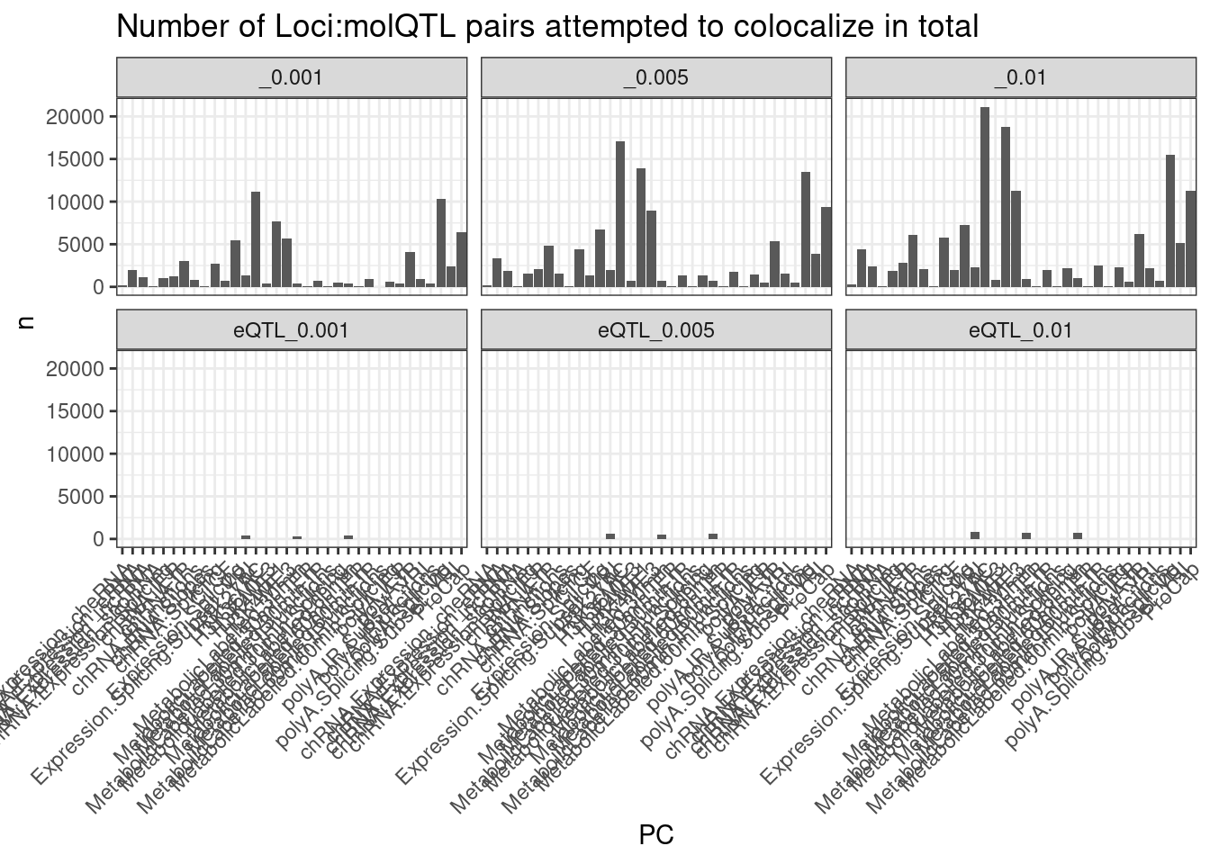
Ok so now make data frame with all attempted coloc pairs (each pair will be representated twice: once with traitA in column1, and once with traitB in column1).
dat.tidy <- dat %>%
  # head(1000) %>%
  unite(Locus, GeneLocus, Threshold, sep = ":") %>%
  left_join(., ., by = "Locus") %>%
    filter(Trait.x != Trait.y) %>%
    separate(Trait.x, into = c("PC1","P1"), sep = "[, ;]", remove=F) %>%
    separate(Trait.y, into = c("PC2","P2"), sep = "[, ;]", remove=F) %>%
    rowwise() %>%
    mutate(PC_ClassPair = paste(PC1, PC2)) %>%
    ungroup() %>%
    # pull(PC_ClassPair) %>% unique()
    mutate(IsColocalizedPair = HyprcolocIteration.x == HyprcolocIteration.y) %>%
    replace_na(list(IsColocalizedPair = FALSE))

RNASeqPhenotypes <- c("MetabolicLabelled.30min", "MetabolicLabelled.60min", "Expression.Splicing.Subset_YRI", "chRNA.Expression.Splicing", "H3K36ME3")


dat.tidy %>%
  filter((PC1 %in% RNASeqPhenotypes) & (PC2 %in% RNASeqPhenotypes)) %>%
  separate(Locus, into=c("Locus", "Threshold"), sep = ":") %>%
  group_by(PC1, PC2, Threshold) %>%
  summarise(FractionColocs = sum(IsColocalizedPair)/n()) %>%
  ungroup() %>%
  mutate(TopPCs = paste(PC1, PC2)) %>%
  mutate(BottomPCs = paste(PC2, PC1)) %>%
  select(-PC1, -PC2) %>%
  gather(key = "MatrixHalf", value = "PCs", TopPCs, BottomPCs) %>%
  separate(PCs, into=c("PC1", "PC2"), sep = " ") %>%
  distinct(PC1, PC2, FractionColocs, Threshold, .keep_all = T) %>%
  ggplot(aes(x=PC1, y=PC2, fill=FractionColocs)) +
  geom_raster() +
  geom_text(aes(label=signif(FractionColocs, 2))) +
  scale_fill_viridis(option="B", direction = 1, limits=c(0.5,1)) +
  facet_wrap(~Threshold) +
  theme_classic() +
  theme(axis.text.x = element_text(angle = 90, vjust = 0.5, hjust=1))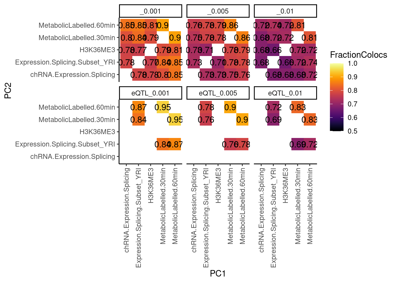
Alternate computation of the same data… How many xQTLs coloc with at least one yQTL:
RecodeVec <- RecodeDat %>%
  select(PC, ShorterAlias) %>%
  deframe()

RecodeIncludePCs <- RecodeDat %>%
  filter(Include) %>%
  pull(PC)


NumQTLs <- dat.tidy %>%
  filter(PC1 %in% RNASeqPhenotypes) %>%
  mutate(PC1 = recode(PC1, !!!RecodeVec)) %>%
  mutate(PC2 = recode(PC2, !!!RecodeVec)) %>%
  separate(Locus, into=c("Locus", "Threshold"), sep = ":") %>%
  distinct(Locus, Threshold, PC1, P1) %>%
  count(Threshold, PC1)


dat.tidy %>%
  filter(PC1 %in% RNASeqPhenotypes) %>%
  filter(PC2 %in% RNASeqPhenotypes) %>%
  mutate(PC1 = recode(PC1, !!!RecodeVec)) %>%
  mutate(PC2 = recode(PC2, !!!RecodeVec)) %>%
  filter(IsColocalizedPair) %>%
  separate(Locus, into=c("Locus", "Threshold"), sep = ":") %>%
  # filter(Locus=="ENSG00000000457.14" & Threshold=="_0.001" & PC1 == "MetabolicLabelled.30min" & P1 =="ENSG00000000457.14" & PC2=="MetabolicLabelled.60min") %>%
  mutate(PC2 = as.factor(PC2)) %>%
  count(Locus, Threshold, PC1, P1, PC2, .drop=F) %>%
  mutate(ContainsAtleastOneColoc = n>0) %>%
  # add_count(PC1, Threshold, wt=, name="NumQTLsInPC1") %>%
  group_by(PC1, PC2, Threshold) %>%
  summarise(SumPC1sWithAtLeast1PC2Coloc = sum(ContainsAtleastOneColoc)) %>%
  left_join(NumQTLs, by=c("Threshold", "PC1")) %>%
  mutate(FractionColocs = SumPC1sWithAtLeast1PC2Coloc/n) %>%
  ggplot(aes(x=PC1, y=PC2, fill=FractionColocs)) +
  geom_raster() +
  geom_text(aes(label=signif(FractionColocs, 2))) +
  scale_fill_viridis(option="B", direction = 1, limits=c(0,1)) +
  facet_wrap(~Threshold) +
  theme_classic() +
  theme(axis.text.x = element_text(angle = 90, vjust = 0.5, hjust=1))
…same thing but with all phenotypes
NumQTLs <- dat.tidy %>%
  filter(PC1 %in% RecodeIncludePCs) %>%
  mutate(PC1 = recode(PC1, !!!RecodeVec)) %>%
  mutate(PC2 = recode(PC2, !!!RecodeVec)) %>%  separate(Locus, into=c("Locus", "Threshold"), sep = ":") %>%
  distinct(Locus, Threshold, PC1, P1) %>%
  count(Threshold, PC1)


dat.tidy %>%
  filter(PC1 %in% RecodeIncludePCs) %>%
  filter(PC2 %in% RecodeIncludePCs) %>%
  mutate(PC1 = recode(PC1, !!!RecodeVec)) %>%
  mutate(PC2 = recode(PC2, !!!RecodeVec)) %>%
  filter(IsColocalizedPair) %>%
  separate(Locus, into=c("Locus", "Threshold"), sep = ":") %>%
  # filter((PC1 %in% RNASeqPhenotypes) & (PC2 %in% RNASeqPhenotypes)) %>%
  mutate(PC2 = as.factor(PC2)) %>%
  count(Locus, Threshold, PC1, P1, PC2, .drop=F) %>%
  mutate(ContainsAtleastOneColoc = n>0) %>%
  # add_count(PC1, Threshold, wt=, name="NumQTLsInPC1") %>%
  group_by(PC1, PC2, Threshold) %>%
  summarise(SumPC1sWithAtLeast1PC2Coloc = sum(ContainsAtleastOneColoc)) %>%
  left_join(NumQTLs, by=c("Threshold", "PC1")) %>%
  # filter(Threshold == "_0.001") %>%
  mutate(FractionColocs = SumPC1sWithAtLeast1PC2Coloc/n) %>%
  ggplot(aes(x=PC1, y=PC2, fill=FractionColocs)) +
  geom_raster() +
  # geom_text(aes(label=signif(FractionColocs*100, 2)), color="blue") +
  scale_fill_viridis(option="B", direction = 1, limits=c(0,1)) +
  facet_wrap(~Threshold) +
  theme_classic() +
  theme(axis.text.x = element_text(angle = 90, vjust = 0.5, hjust=1))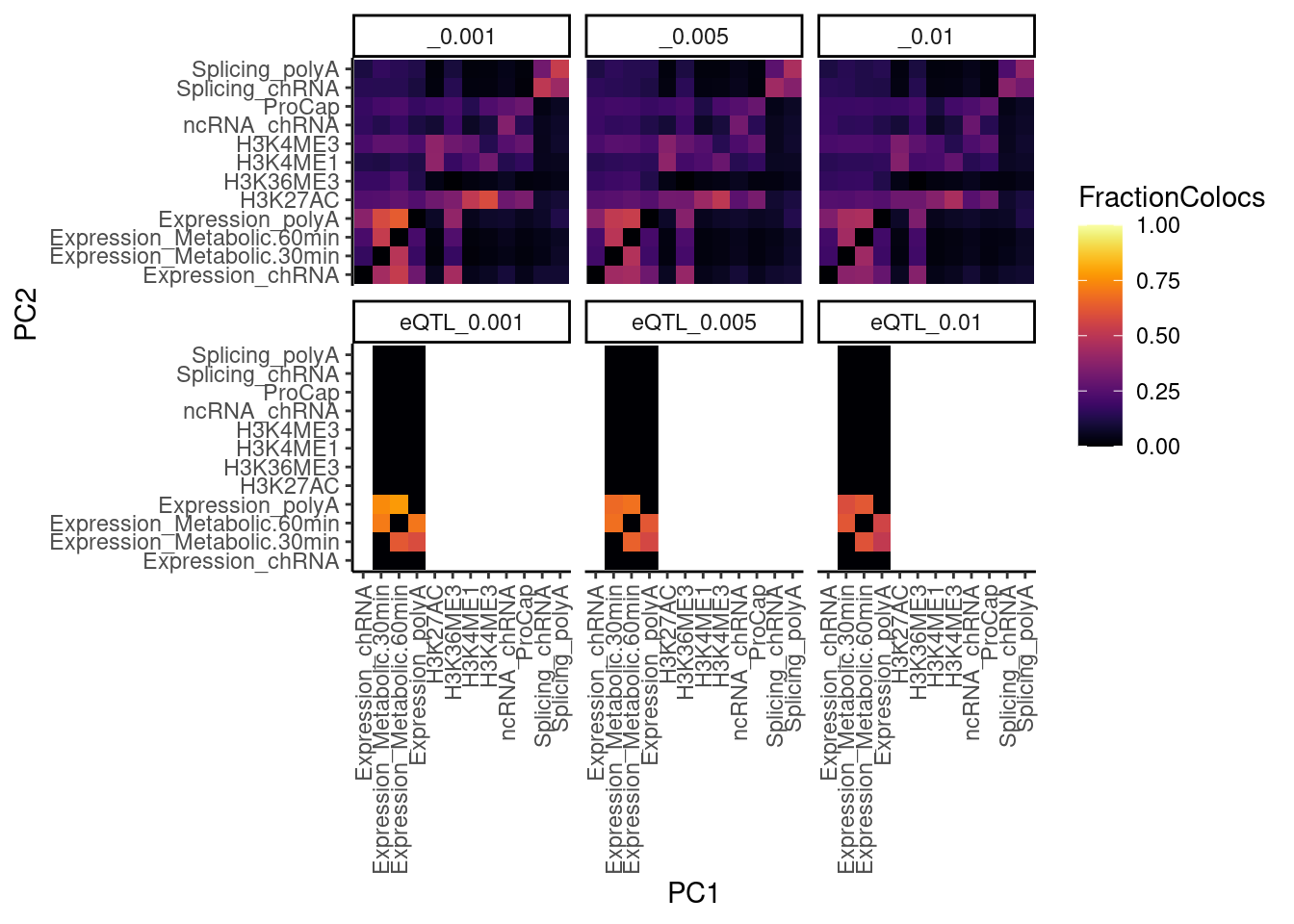
dat.tidy %>%
  filter(PC1 %in% RecodeIncludePCs) %>%
  filter(PC2 %in% RecodeIncludePCs) %>%
  mutate(PC1 = recode(PC1, !!!RecodeVec)) %>%
  mutate(PC2 = recode(PC2, !!!RecodeVec)) %>%
  filter(IsColocalizedPair) %>%
  separate(Locus, into=c("Locus", "Threshold"), sep = ":") %>%
  # filter((PC1 %in% RNASeqPhenotypes) & (PC2 %in% RNASeqPhenotypes)) %>%
  mutate(PC2 = as.factor(PC2)) %>%
  count(Locus, Threshold, PC1, P1, PC2, .drop=F) %>%
  mutate(ContainsAtleastOneColoc = n>0) %>%
  # add_count(PC1, Threshold, wt=, name="NumQTLsInPC1") %>%
  group_by(PC1, PC2, Threshold) %>%
  summarise(SumPC1sWithAtLeast1PC2Coloc = sum(ContainsAtleastOneColoc)) %>%
  left_join(NumQTLs, by=c("Threshold", "PC1")) %>%
  filter(Threshold == "_0.001") %>%
  mutate(FractionColocs = SumPC1sWithAtLeast1PC2Coloc/n) %>%
  ggplot(aes(x=PC1, y=PC2, fill=FractionColocs)) +
  geom_raster() +
  geom_text(aes(label=signif(FractionColocs*100, 2)), color="blue") +
  scale_fill_viridis(option="B", direction = 1, limits=c(0,1)) +
  facet_wrap(~Threshold) +
  theme_classic() +
  theme(axis.text.x = element_text(angle = 90, vjust = 0.5, hjust=1))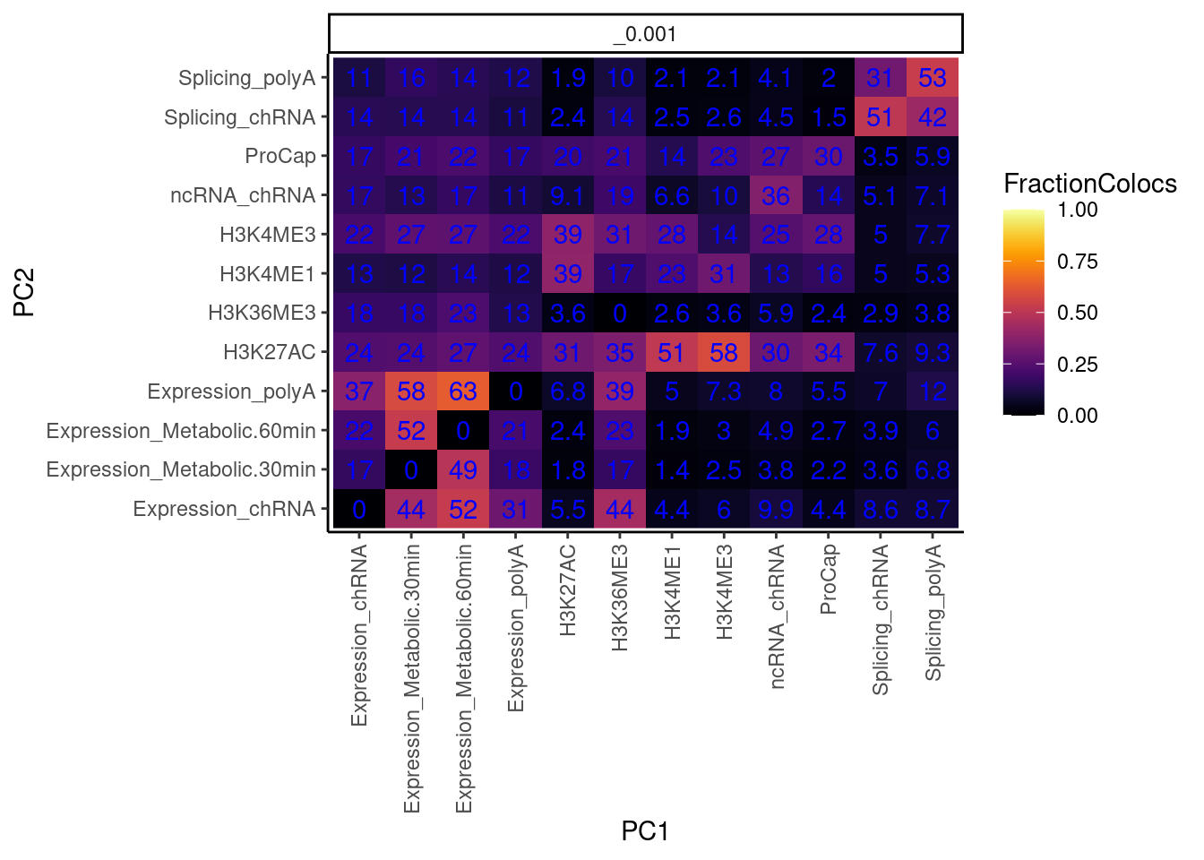
I also want to make this plot distinguishing between promoter chromatin effects and non-promoter effects… for now let me just remake the plot after grouping these different chromatin phenotypes
NumQTLs <- dat.tidy %>%
  filter(PC1 %in% RecodeIncludePCs) %>%
  mutate(PC1 = recode(PC1, !!!RecodeVec)) %>%
  mutate(PC2 = recode(PC2, !!!RecodeVec)) %>%  separate(Locus, into=c("Locus", "Threshold"), sep = ":") %>%
  mutate(PC1 = recode(PC1, H3K4ME3="H3K(4ME3|4ME1|K27AC)", H3K27AC="H3K(4ME3|4ME1|K27AC)", H3K4ME1="H3K(4ME3|4ME1|K27AC)")) %>%
  mutate(PC2 = recode(PC2, H3K4ME3="H3K(4ME3|4ME1|K27AC)", H3K27AC="H3K(4ME3|4ME1|K27AC)", H3K4ME1="H3K(4ME3|4ME1|K27AC)")) %>%
  distinct(Locus, Threshold, PC1, P1) %>%
  count(Threshold, PC1)

dat.tidy %>%
  filter(PC1 %in% RecodeIncludePCs) %>%
  filter(PC2 %in% RecodeIncludePCs) %>%
  mutate(PC1 = recode(PC1, !!!RecodeVec)) %>%
  mutate(PC2 = recode(PC2, !!!RecodeVec)) %>%
  mutate(PC1 = recode(PC1, H3K4ME3="H3K(4ME3|4ME1|K27AC)", H3K27AC="H3K(4ME3|4ME1|K27AC)", H3K4ME1="H3K(4ME3|4ME1|K27AC)")) %>%
  mutate(PC2 = recode(PC2, H3K4ME3="H3K(4ME3|4ME1|K27AC)", H3K27AC="H3K(4ME3|4ME1|K27AC)", H3K4ME1="H3K(4ME3|4ME1|K27AC)")) %>%
  filter(IsColocalizedPair) %>%
  separate(Locus, into=c("Locus", "Threshold"), sep = ":") %>%
  # filter((PC1 %in% RNASeqPhenotypes) & (PC2 %in% RNASeqPhenotypes)) %>%
  mutate(PC2 = as.factor(PC2)) %>%
  count(Locus, Threshold, PC1, P1, PC2, .drop=F) %>%
  mutate(ContainsAtleastOneColoc = n>0) %>%
  # add_count(PC1, Threshold, wt=, name="NumQTLsInPC1") %>%
  group_by(PC1, PC2, Threshold) %>%
  summarise(SumPC1sWithAtLeast1PC2Coloc = sum(ContainsAtleastOneColoc)) %>%
  left_join(NumQTLs, by=c("Threshold", "PC1")) %>%
  filter(Threshold == "_0.001") %>%
  mutate(FractionColocs = SumPC1sWithAtLeast1PC2Coloc/n) %>%
  ggplot(aes(x=PC1, y=PC2, fill=FractionColocs)) +
  geom_raster() +
  geom_text(aes(label=signif(FractionColocs*100, 2)), color="blue") +
  scale_fill_viridis(option="B", direction = 1, limits=c(0,1)) +
  facet_wrap(~Threshold) +
  theme_classic() +
  theme(axis.text.x = element_text(angle = 90, vjust = 0.5, hjust=1))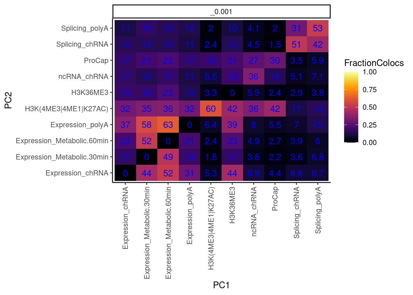
I previously estimated more like 80% of eQTL have chromatin effect. now its more like a third. what gives?
dat.tidy %>%
  filter(PC1 %in% c("Expression.Splicing.Subset_YRI", "chRNA.Expression.Splicing")) %>%
  separate(Locus, into=c("Locus", "Threshold"), sep = ":") %>%
  separate(Threshold, into = c("ColocPhenotypeClass", "Threshold"), sep="_") %>%
  filter(ColocPhenotypeClass == "") %>%
  mutate(GenePeakPair = paste(P1, P2, sep=";")) %>%
  mutate(IsGenePeakPairPromoter = PC2 %in% c("H3K4ME3", "H3K27AC", "H3K4ME1")) %>%
  mutate(IsColocalizedGenePeakPromoter = IsColocalizedPair & IsGenePeakPairPromoter) %>%
  group_by(Locus, P1, PC1, Threshold) %>%
  ## THIS NEXT LINE IS JUST WRONG. IT COUNTS ATTEMPTED COLOCS
  summarise(GeneContainsColocalizedGenePeakPromoter = any(IsGenePeakPairPromoter)) %>%
  group_by(Threshold, PC1) %>%
  summarise(FractionColocs = sum(GeneContainsColocalizedGenePeakPromoter),
            eGenesAttemptedToColoc = n() -  sum(GeneContainsColocalizedGenePeakPromoter)) %>%
  ungroup() %>%
  gather("IsColocalized", "NumberGenes", FractionColocs, eGenesAttemptedToColoc) %>%
  ggplot(aes(x=Threshold, y=NumberGenes, fill=IsColocalized)) +
  geom_col() +
  facet_wrap(~PC1) +
  scale_fill_discrete(labels = c("No", "Yes")) +
  labs(title = "~4/5 eGenes have colocalized chromatin effects somewhere",
       y = str_wrap("Number eGenes", width=30),
       fill = str_wrap("Is eQTL coloc w/ any [H3K4ME1|H3K4ME3|H3K27AC] QTL", width=20)) +
  theme_classic() +
  theme(axis.text.x = element_text(angle = 90, vjust = 0.5, hjust=1))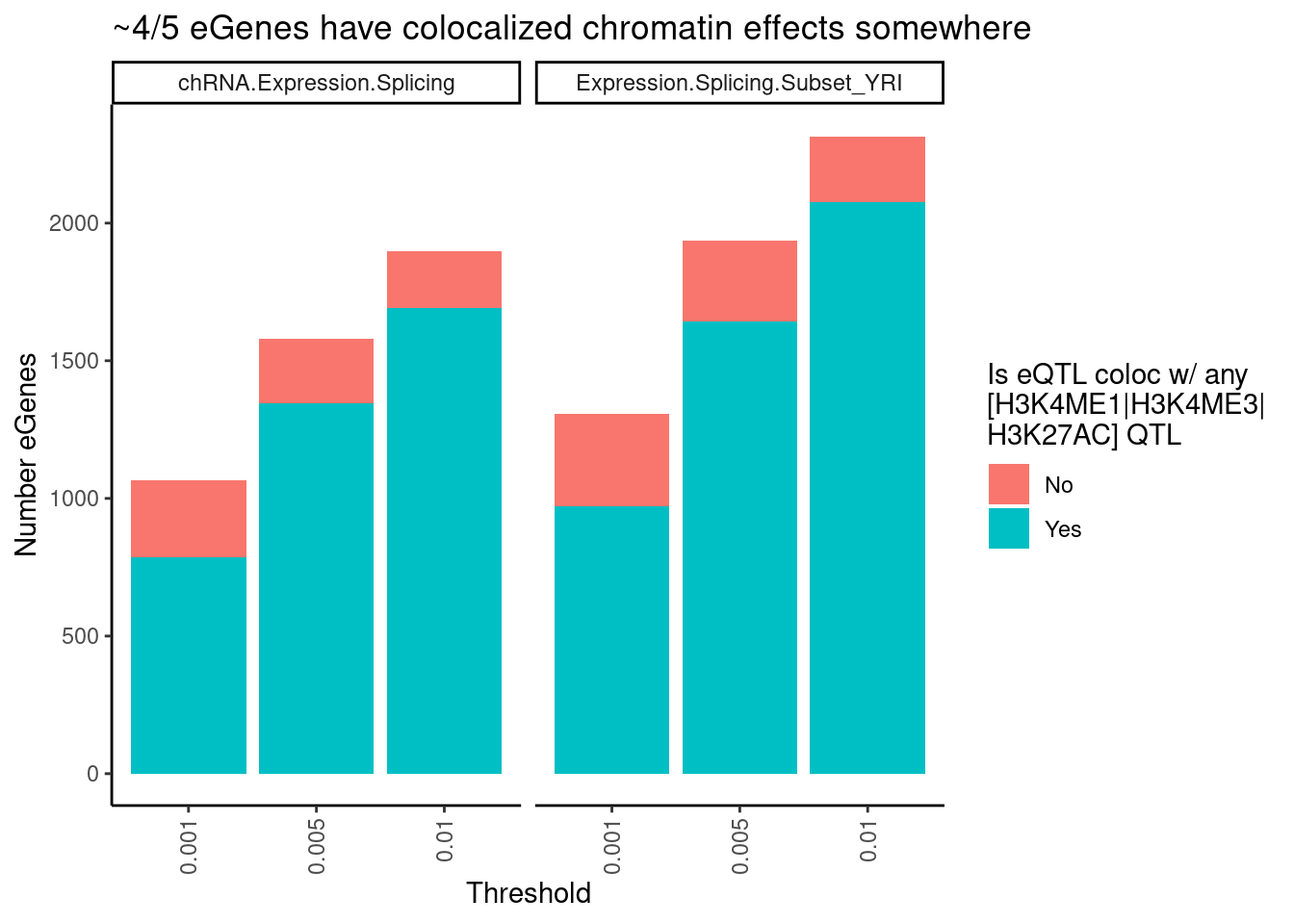
dat.tidy %>%
  filter(PC1 %in% c("Expression.Splicing.Subset_YRI", "chRNA.Expression.Splicing")) %>%
  separate(Locus, into=c("Locus", "Threshold"), sep = ":") %>%
  separate(Threshold, into = c("ColocPhenotypeClass", "Threshold"), sep="_") %>%
  filter(ColocPhenotypeClass == "") %>%
  mutate(GenePeakPair = paste(P1, P2, sep=";")) %>%
  mutate(IsGenePeakPairPromoter = PC2 %in% c("H3K4ME3", "H3K27AC", "H3K4ME1")) %>%
  mutate(IsColocalizedGenePeakPromoter = IsColocalizedPair & IsGenePeakPairPromoter) %>%
  group_by(Locus, P1, PC1, Threshold) %>%
  ## THIS NEXT LINE CORRECT NOW. IT COUNTS COLOCS
  summarise(GeneContainsColocalizedGenePeakPromoter = any(IsColocalizedGenePeakPromoter)) %>%
  group_by(Threshold, PC1) %>%
  summarise(FractionColocs = sum(GeneContainsColocalizedGenePeakPromoter),
            eGenesAttemptedToColoc = n() -  sum(GeneContainsColocalizedGenePeakPromoter)) %>%
  ungroup() %>%
  gather("IsColocalized", "NumberGenes", FractionColocs, eGenesAttemptedToColoc) %>%
  ggplot(aes(x=Threshold, y=NumberGenes, fill=IsColocalized)) +
  geom_col() +
  facet_wrap(~PC1) +
  scale_fill_discrete(labels = c("No", "Yes")) +
  labs(title = "~1/3 eGenes have colocalized chromatin effects somewhere",
       y = str_wrap("Number eGenes", width=30),
       fill = str_wrap("Is eQTL coloc w/ any [H3K4ME1|H3K4ME3|H3K27AC] QTL", width=20)) +
  theme_classic() +
  theme(axis.text.x = element_text(angle = 90, vjust = 0.5, hjust=1))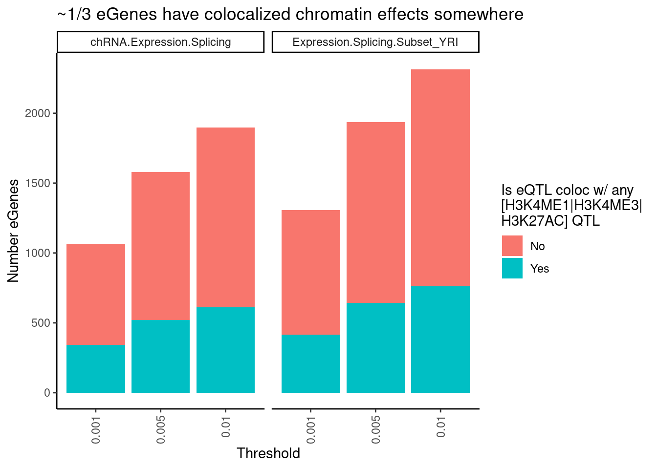
PeaksToTSS <- Sys.glob("../code/Misc/PeaksClosestToTSS/*_assigned.tsv.gz") %>%
  setNames(str_replace(., "../code/Misc/PeaksClosestToTSS/(.+?)_assigned.tsv.gz", "\\1")) %>%
  lapply(read_tsv) %>%
  bind_rows(.id="ChromatinMark") %>%
  mutate(GenePeakPair = paste(gene, peak, sep = ";"))
Parsed with column specification:
cols(
chrom = col_character(),
TSS_start = col_double(),
gene = col_character(),
strand = col_character(),
peak = col_character(),
distance = col_double()
)
Parsed with column specification:
cols(
chrom = col_character(),
TSS_start = col_double(),
gene = col_character(),
strand = col_character(),
peak = col_character(),
distance = col_double()
)
Parsed with column specification:
cols(
chrom = col_character(),
TSS_start = col_double(),
gene = col_character(),
strand = col_character(),
peak = col_character(),
distance = col_double()
)dat.tidy %>%
filter(PC1 %in% c("Expression.Splicing.Subset_YRI", "chRNA.Expression.Splicing")) %>%
separate(Locus, into=c("Locus", "Threshold"), sep = ":") %>%
separate(Threshold, into = c("ColocPhenotypeClass", "Threshold"), sep="_") %>%
filter(ColocPhenotypeClass == "") %>%
mutate(GenePeakPair = paste(P1, P2, sep=";")) %>%
mutate(IsGenePeakPairPromoter = GenePeakPair %in% PeaksToTSS$GenePeakPair) %>%
mutate(IsColocalizedGenePeakPromoter = IsColocalizedPair & IsGenePeakPairPromoter) %>%
group_by(Locus, P1, PC1, Threshold) %>%
summarise(GeneContainsColocalizedGenePeakPromoter = any(IsColocalizedGenePeakPromoter)) %>%
group_by(Threshold, PC1) %>%
summarise(FractionColocs = sum(GeneContainsColocalizedGenePeakPromoter),
eGenesAttemptedToColoc = n() - sum(GeneContainsColocalizedGenePeakPromoter)) %>%
ungroup() %>%
gather("IsColocalized", "NumberGenes", FractionColocs, eGenesAttemptedToColoc) %>%
ggplot(aes(x=Threshold, y=NumberGenes, fill=IsColocalized)) +
geom_col() +
facet_wrap(~PC1) +
scale_fill_discrete(labels = c("Yes", "No")) +
labs(title = "~1/4 eGenes have colocalized chromatin effects at promoter",
y = str_wrap("Number eGenes", width=30),
fill = str_wrap("Is eQTL coloc w/ [H3K4ME1|H3K4ME3|H3K27AC] QTL at promoter", width=20)) +
theme_classic() +
theme(axis.text.x = element_text(angle = 90, vjust = 0.5, hjust=1))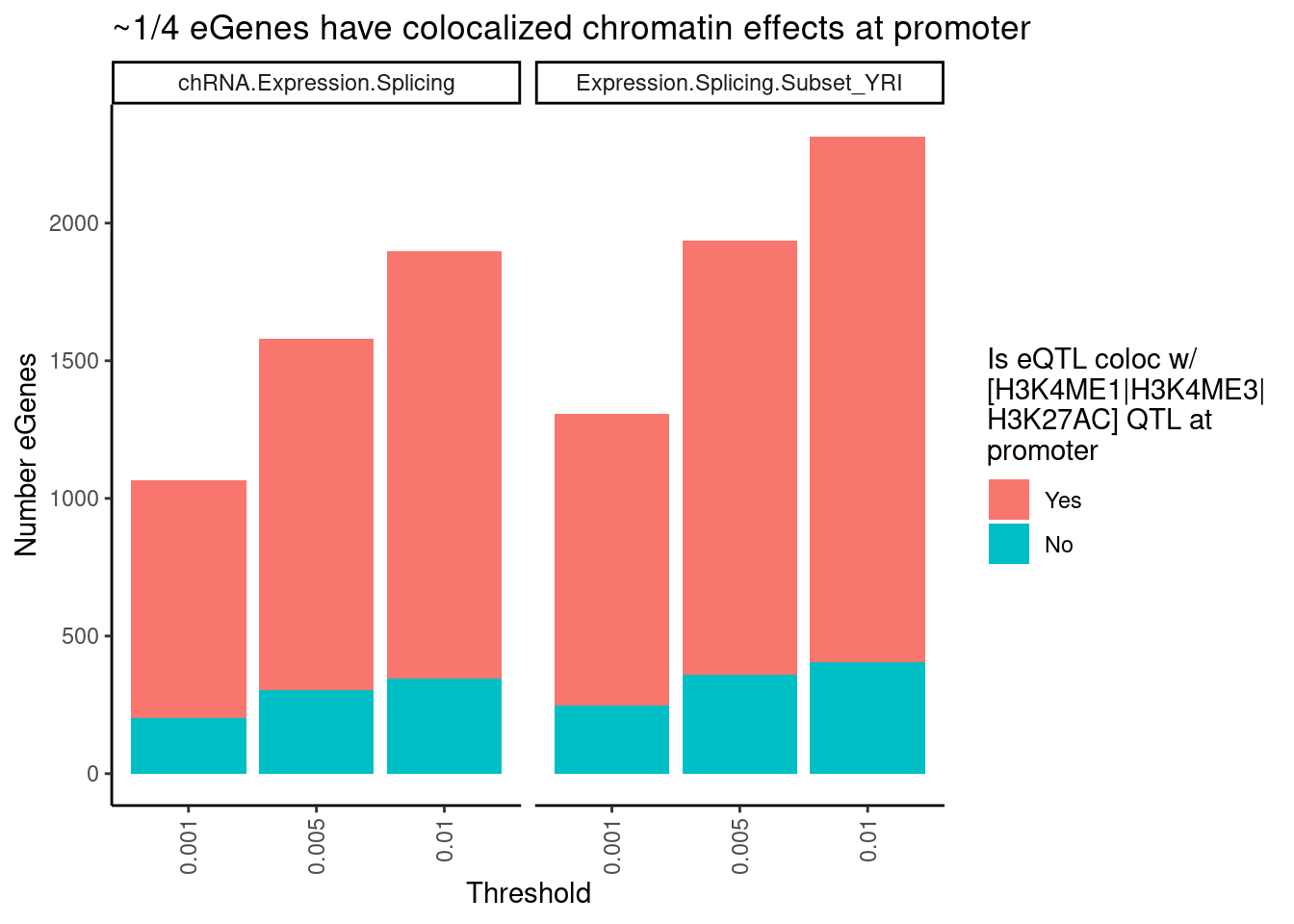
PeaksToTSS# A tibble: 255,075 x 8
ChromatinMark chrom TSS_start gene strand peak distance GenePeakPair
<chr> <chr> <dbl> <chr> <chr> <chr> <dbl> <chr>
1 H3K27AC chr1 29552 ENSG0… + H3K27… 0 ENSG0000024…
2 H3K27AC chr1 29569 ENSG0… - H3K27… 0 ENSG0000022…
3 H3K27AC chr1 30265 ENSG0… + H3K27… -254 ENSG0000024…
4 H3K27AC chr1 30364 ENSG0… + H3K27… -353 ENSG0000028…
5 H3K27AC chr1 629060 ENSG0… + H3K27… 121 ENSG0000022…
6 H3K27AC chr1 629638 ENSG0… + H3K27… 0 ENSG0000022…
7 H3K27AC chr1 631072 ENSG0… + H3K27… 0 ENSG0000023…
8 H3K27AC chr1 631149 ENSG0… - H3K27… 0 ENSG0000023…
9 H3K27AC chr1 631203 ENSG0… - H3K27… 0 ENSG0000023…
10 H3K27AC chr1 632412 ENSG0… - H3K27… 0 ENSG0000027…
# … with 255,065 more rowsNumQTLs <- dat.tidy %>%
filter(PC1 %in% RecodeIncludePCs) %>%
mutate(PC1 = recode(PC1, !!!RecodeVec)) %>%
mutate(PC2 = recode(PC2, !!!RecodeVec)) %>% separate(Locus, into=c("Locus", "Threshold"), sep = ":") %>%
mutate(PC1 = recode(PC1, H3K4ME3="H3K(4ME3|4ME1|K27AC)", H3K27AC="H3K(4ME3|4ME1|K27AC)", H3K4ME1="H3K(4ME3|4ME1|K27AC)")) %>%
mutate(PC2 = recode(PC2, H3K4ME3="H3K(4ME3|4ME1|K27AC)", H3K27AC="H3K(4ME3|4ME1|K27AC)", H3K4ME1="H3K(4ME3|4ME1|K27AC)")) %>%
distinct(Locus, Threshold, PC1, P1) %>%
count(Threshold, PC1)
dat.tidy %>%
filter(PC1 %in% RecodeIncludePCs) %>%
filter(PC2 %in% RecodeIncludePCs) %>%
mutate(PC1 = recode(PC1, !!!RecodeVec)) %>%
mutate(PC2 = recode(PC2, !!!RecodeVec)) %>%
mutate(PC1 = recode(PC1, H3K4ME3="H3K(4ME3|4ME1|K27AC)", H3K27AC="H3K(4ME3|4ME1|K27AC)", H3K4ME1="H3K(4ME3|4ME1|K27AC)")) %>%
mutate(PC2 = recode(PC2, H3K4ME3="H3K(4ME3|4ME1|K27AC)", H3K27AC="H3K(4ME3|4ME1|K27AC)", H3K4ME1="H3K(4ME3|4ME1|K27AC)")) %>%
filter(IsColocalizedPair) %>%
separate(Locus, into=c("Locus", "Threshold"), sep = ":") %>%
mutate(PC2 = case_when(
paste(Locus, P2, sep=';') %in% PeaksToTSS$GenePeakPair ~ "H3K(4ME3|4ME1|K27AC) @ Promoter",
PC2=="H3K(4ME3|4ME1|K27AC)" ~ "H3K(4ME3|4ME1|K27AC) Elsewhere",
TRUE ~ PC2
)) %>%
mutate(PC2 = as.factor(PC2)) %>%
count(Locus, Threshold, PC1, P1, PC2, .drop=F) %>%
mutate(ContainsAtleastOneColoc = n>0) %>%
group_by(PC1, PC2, Threshold) %>%
summarise(SumPC1sWithAtLeast1PC2Coloc = sum(ContainsAtleastOneColoc)) %>%
left_join(NumQTLs, by=c("Threshold", "PC1")) %>%
filter(Threshold == "_0.001") %>%
mutate(FractionColocs = SumPC1sWithAtLeast1PC2Coloc/n) %>%
ggplot(aes(x=PC1, y=PC2, fill=FractionColocs)) +
geom_raster() +
geom_text(aes(label=signif(FractionColocs*100, 2)), color="blue") +
scale_fill_viridis(option="B", direction = 1, limits=c(0,1)) +
facet_wrap(~Threshold) +
theme_classic() +
theme(axis.text.x = element_text(angle = 90, vjust = 0.5, hjust=1))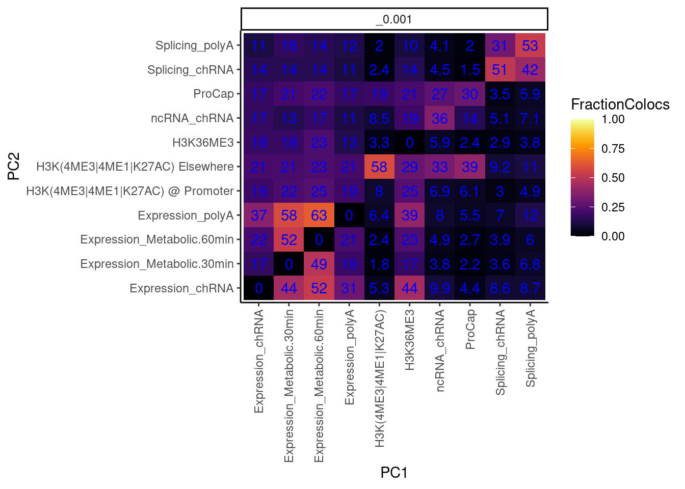
Check if IR methods are picking up on eQTL. I think the biological ones we want to capture will generally have negative effect size correlations (increased IR –> decreased expression)… The ones that are just picking up on eQTLs will mostly be positive effect ize correlations.
dat.effectsizes <- Sys.glob("../code/hyprcoloc/Results/ForColoc/MolColocTest*_*/tidy_results_OnlyColocalized.txt.gz") %>%
  setNames(str_replace(., "../code/hyprcoloc/Results/ForColoc/MolColocTest(.*?)_(.+?)/tidy_results_OnlyColocalized.txt.gz", "\\1_0.\\2")) %>%
  lapply(read_tsv) %>%
  bind_rows(.id="Threshold")
Parsed with column specification:
cols(
snp = col_character(),
beta = col_double(),
beta_se = col_double(),
p = col_double(),
Locus = col_character(),
phenotype_full = col_character(),
iteration = col_double(),
ColocPr = col_double(),
RegionalPr = col_double(),
TopSNPFinemapPr = col_double()
)
Parsed with column specification:
cols(
snp = col_character(),
beta = col_double(),
beta_se = col_double(),
p = col_double(),
Locus = col_character(),
phenotype_full = col_character(),
iteration = col_double(),
ColocPr = col_double(),
RegionalPr = col_double(),
TopSNPFinemapPr = col_double()
)
Parsed with column specification:
cols(
snp = col_character(),
beta = col_double(),
beta_se = col_double(),
p = col_double(),
Locus = col_character(),
phenotype_full = col_character(),
iteration = col_double(),
ColocPr = col_double(),
RegionalPr = col_double(),
TopSNPFinemapPr = col_double()
)
Parsed with column specification:
cols(
snp = col_character(),
beta = col_double(),
beta_se = col_double(),
p = col_double(),
Locus = col_character(),
phenotype_full = col_character(),
iteration = col_double(),
ColocPr = col_double(),
RegionalPr = col_double(),
TopSNPFinemapPr = col_double()
)
Parsed with column specification:
cols(
snp = col_character(),
beta = col_double(),
beta_se = col_double(),
p = col_double(),
Locus = col_character(),
phenotype_full = col_character(),
iteration = col_double(),
ColocPr = col_double(),
RegionalPr = col_double(),
TopSNPFinemapPr = col_double()
)
Parsed with column specification:
cols(
snp = col_character(),
beta = col_double(),
beta_se = col_double(),
p = col_double(),
Locus = col_character(),
phenotype_full = col_character(),
iteration = col_double(),
ColocPr = col_double(),
RegionalPr = col_double(),
TopSNPFinemapPr = col_double()
)dat.tidy.witheffects <- dat %>%
left_join(
dat.effectsizes %>%
select(GeneLocus=Locus, TopCandidateSNP=snp, Trait=phenotype_full, Threshold, beta, beta_se, p)
, by=c("GeneLocus", "TopCandidateSNP", "Threshold", "Trait")) %>%
unite(Locus, GeneLocus, Threshold, sep = ":") %>%
left_join(., ., by = "Locus") %>%
filter(Trait.x != Trait.y) %>%
separate(Trait.x, into = c("PC1","P1"), sep = "[, ;]", remove=F) %>%
separate(Trait.y, into = c("PC2","P2"), sep = "[, ;]", remove=F) %>%
rowwise() %>%
mutate(PC_ClassPair = paste(PC1, PC2)) %>%
ungroup() %>%
# pull(PC_ClassPair) %>% unique()
mutate(IsColocalizedPair = HyprcolocIteration.x == HyprcolocIteration.y) %>%
replace_na(list(IsColocalizedPair = FALSE))
dat.tidy.witheffects %>%
filter(IsColocalizedPair) %>%
separate(Locus, into=c("Locus", "Threshold"), sep = ":") %>%
filter(Threshold == "_0.001") %>%
group_by(PC1, PC2) %>%
summarise(cor = cor(beta.x, beta.y, method="spearman")) %>%
pivot_wider(names_from = "PC1", values_from = "cor", values_fill=NA, names_sort=T) %>%
column_to_rownames("PC2") %>%
as.matrix() %>%
heatmap.2(trace="none", col=colorpanel(75, "blue", "black", "yellow"), cexRow = 1, cexCol = 1, offsetRow=0, offsetCol = 0, margins=c(11,11), dendrogram = "column")Warning in cor(beta.x, beta.y, method = "spearman"): the standard deviation
is zero
Warning in cor(beta.x, beta.y, method = "spearman"): the standard deviation
is zero
Warning in cor(beta.x, beta.y, method = "spearman"): the standard deviation
is zero
Warning in cor(beta.x, beta.y, method = "spearman"): the standard deviation
is zero
Warning in cor(beta.x, beta.y, method = "spearman"): the standard deviation
is zero
Warning in cor(beta.x, beta.y, method = "spearman"): the standard deviation
is zero
Warning in cor(beta.x, beta.y, method = "spearman"): the standard deviation
is zero
Warning in cor(beta.x, beta.y, method = "spearman"): the standard deviation
is zero
Warning in cor(beta.x, beta.y, method = "spearman"): the standard deviation
is zero
Warning in cor(beta.x, beta.y, method = "spearman"): the standard deviation
is zero
Warning in cor(beta.x, beta.y, method = "spearman"): the standard deviation
is zero
Warning in cor(beta.x, beta.y, method = "spearman"): the standard deviation
is zero
Warning in cor(beta.x, beta.y, method = "spearman"): the standard deviation
is zero
Warning in cor(beta.x, beta.y, method = "spearman"): the standard deviation
is zero
Warning in cor(beta.x, beta.y, method = "spearman"): the standard deviation
is zero
Warning in cor(beta.x, beta.y, method = "spearman"): the standard deviation
is zero
Warning in cor(beta.x, beta.y, method = "spearman"): the standard deviation
is zero
Warning in cor(beta.x, beta.y, method = "spearman"): the standard deviation
is zero
Warning in cor(beta.x, beta.y, method = "spearman"): the standard deviation
is zero
Warning in cor(beta.x, beta.y, method = "spearman"): the standard deviation
is zero
Warning in cor(beta.x, beta.y, method = "spearman"): the standard deviation
is zero
Warning in cor(beta.x, beta.y, method = "spearman"): the standard deviation
is zero
Warning in cor(beta.x, beta.y, method = "spearman"): the standard deviation
is zero
Warning in cor(beta.x, beta.y, method = "spearman"): the standard deviation
is zero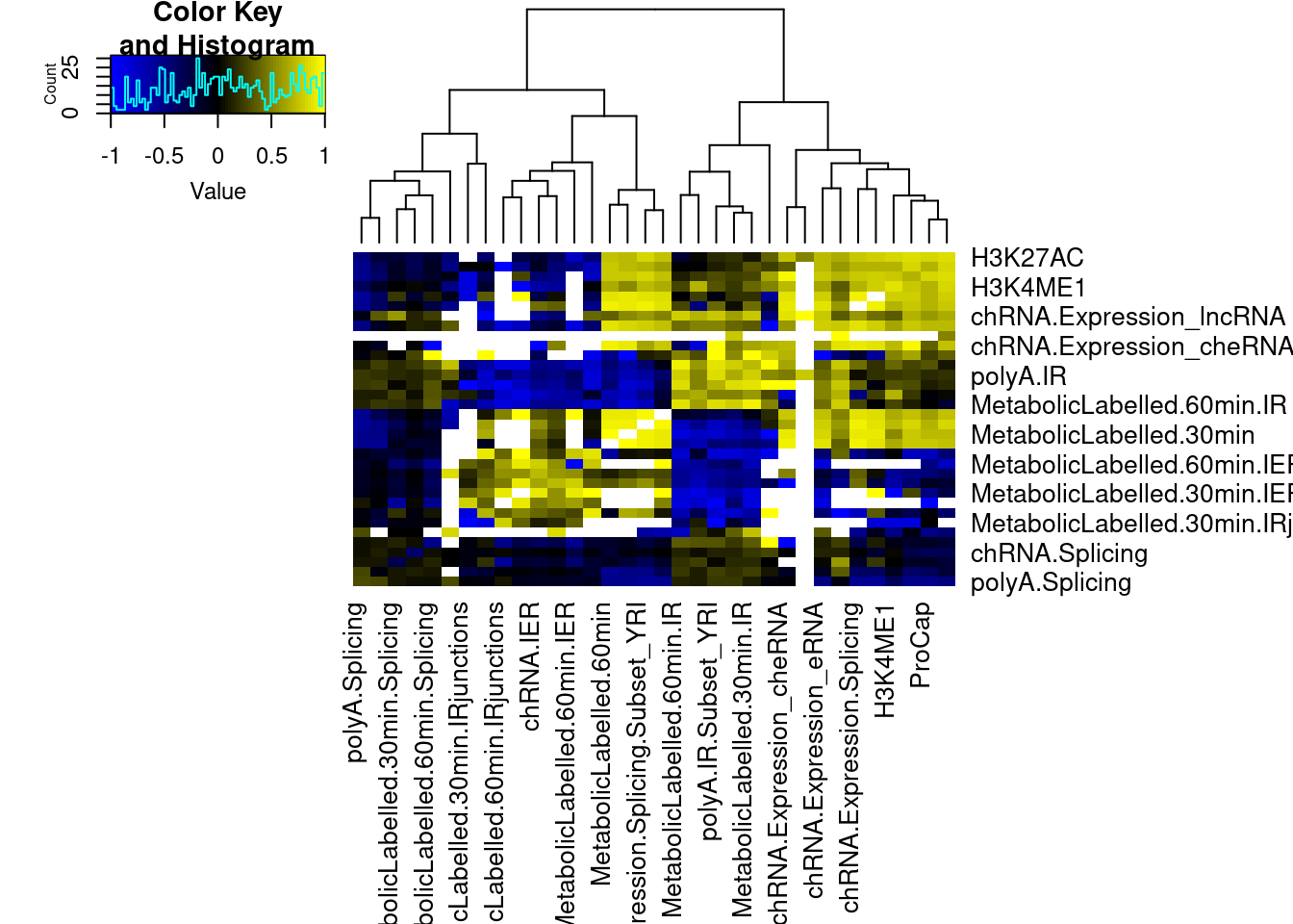
sessionInfo()R version 3.6.1 (2019-07-05)
Platform: x86_64-pc-linux-gnu (64-bit)
Running under: Scientific Linux 7.4 (Nitrogen)
Matrix products: default
BLAS/LAPACK: /software/openblas-0.2.19-el7-x86_64/lib/libopenblas_haswellp-r0.2.19.so
locale:
[1] LC_CTYPE=en_US.UTF-8 LC_NUMERIC=C
[3] LC_TIME=en_US.UTF-8 LC_COLLATE=en_US.UTF-8
[5] LC_MONETARY=en_US.UTF-8 LC_MESSAGES=en_US.UTF-8
[7] LC_PAPER=en_US.UTF-8 LC_NAME=C
[9] LC_ADDRESS=C LC_TELEPHONE=C
[11] LC_MEASUREMENT=en_US.UTF-8 LC_IDENTIFICATION=C
attached base packages:
[1] stats graphics grDevices utils datasets methods base
other attached packages:
[1] qvalue_2.16.0 data.table_1.14.2 gplots_3.0.1.1
[4] viridis_0.5.1 viridisLite_0.3.0 forcats_0.4.0
[7] stringr_1.4.0 dplyr_0.8.3 purrr_0.3.4
[10] readr_1.3.1 tidyr_1.1.0 tibble_2.1.3
[13] ggplot2_3.3.5 tidyverse_1.3.0
loaded via a namespace (and not attached):
[1] Rcpp_1.0.5 lubridate_1.7.4 lattice_0.20-38
[4] gtools_3.8.1 utf8_1.1.4 assertthat_0.2.1
[7] rprojroot_2.0.2 digest_0.6.20 plyr_1.8.4
[10] R6_2.4.0 cellranger_1.1.0 backports_1.1.4
[13] reprex_0.3.0 evaluate_0.14 httr_1.4.1
[16] pillar_1.4.2 rlang_0.4.10 readxl_1.3.1
[19] rstudioapi_0.10 gdata_2.18.0 rmarkdown_1.13
[22] labeling_0.3 splines_3.6.1 munsell_0.5.0
[25] broom_0.5.2 compiler_3.6.1 httpuv_1.5.1
[28] modelr_0.1.8 xfun_0.8 pkgconfig_2.0.2
[31] htmltools_0.3.6 tidyselect_1.1.0 gridExtra_2.3
[34] workflowr_1.6.2 fansi_0.4.0 crayon_1.3.4
[37] dbplyr_1.4.2 withr_2.4.1 later_0.8.0
[40] bitops_1.0-6 grid_3.6.1 nlme_3.1-140
[43] jsonlite_1.6 gtable_0.3.0 lifecycle_0.1.0
[46] DBI_1.1.0 git2r_0.26.1 magrittr_1.5
[49] scales_1.1.0 KernSmooth_2.23-15 cli_2.2.0
[52] stringi_1.4.3 farver_2.1.0 reshape2_1.4.3
[55] fs_1.3.1 promises_1.0.1 xml2_1.3.2
[58] ellipsis_0.2.0.1 generics_0.0.2 vctrs_0.3.1
[61] tools_3.6.1 glue_1.3.1 hms_0.5.3
[64] yaml_2.2.0 colorspace_1.4-1 caTools_1.17.1.2
[67] rvest_0.3.5 knitr_1.23 haven_2.3.1